Neural Radiance Field
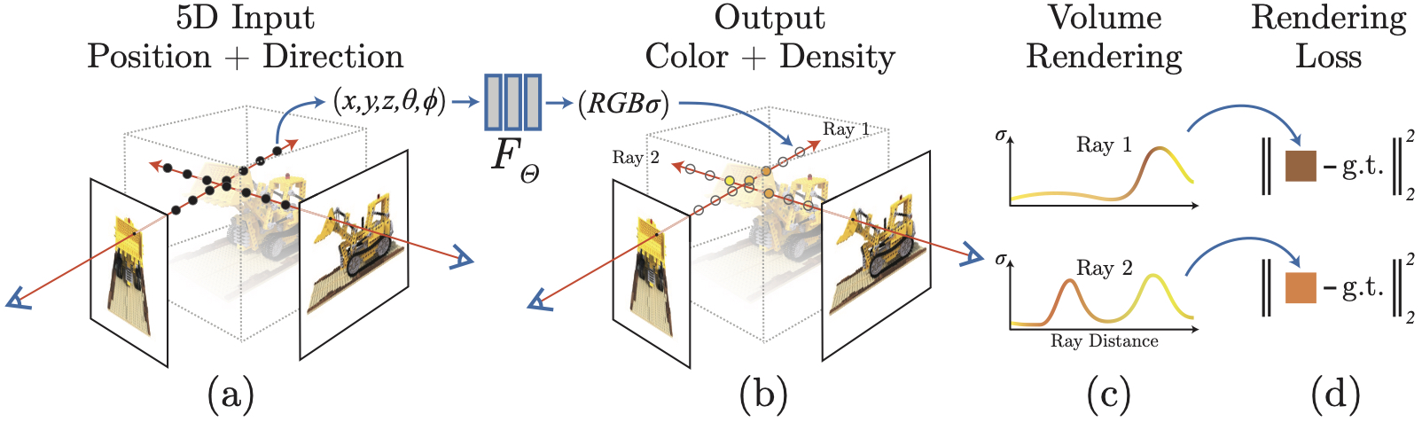
[cnn mlp nerf deep-learning differential-rendering Neural Radiance Field (NeRF), you may have heard words many times for the past few months. Yes, this is the latest progress of neutral work and computer graphics. NeRF represents a scene with learned, continuous volumetric radiance field \(F_{\theta}\) defined over a bounded 3D volume. In Nerf, \(F_{\theta}\) is a multilayer perceptron (MLP) that takes as input a 3D position \(x=(x,y,z)\) and unit-norm viewing direction \(d=(d_x,d_y,d_z)\), and produces as output a density \(\sigma\) and color \(c=(r,g,b)\). By enumerating all most position and direction for a bounded 3D volumne, we could obtain the 3D scene.
The weights of the multilayer perceptron that parameterize \(F_{\theta}\) are optimized so as to encode the radiance field of the scene. Volume rendering is used to compute the color of a single pixel.
The first well known paper on this topic is NeRF: Representing Scenes as Neural Radiance Fields for View Synthesis. To learn such field, you only need to capture a few images of the scene from different angles (a), then you try to fit the MLP between your camera pose to the image(b). This is also illustrated in the chart below.
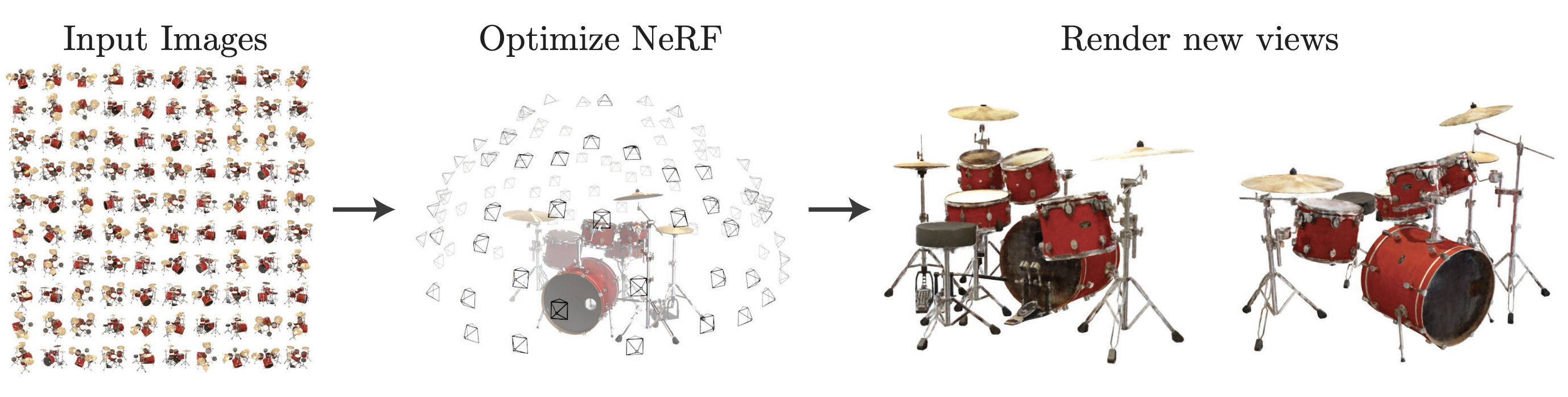
For rendering a scene (i.e., inference, c), you need to pick a camera view, which is 3D position and orientation. Then you enumerate the directions according the orientation of the camera and the angle of view of the camera, to estimate the brightness and color for this direction. Putting all together you got an image for this camera view.
More on Training
The training aims to learn the MLP (weights) such that the volume generated by the MLP could render the images replicating the input images. To this end, MLP will produce color and volume density by enumerating the rays over all position and direction. Then images will be rendered from this color and volume density at the same camera view as the input images. Given this whole process (including rendering) is differentiable, we could optimize the MLP such that the differences of rendered images and input images are minimized.
You may realize the training requires to have the correspondence between the input (3D locations and directions) and the output (pixel intensity and density). The output is easily available from the images. But for the input, 3D locations and directions, you would need to have camera extrinic and intrinsic.
Camera extrinsic could be computed via struction from motion. The NeRF paper recommend using the imgs2poses.py script from the LLFF code. Combining camera intrinsic and extrinsic, you could obtain the orientation of each ray from camera to every pixels on the image.
Positional Encoding
We find that the basic implementation of optimizing a neural radiance field representation for a complex scene does not converge to a sufficiently high- resolution representation and is inefficient in the required number of samples per camera ray. We address these issues by transforming input 5D coordinates with a positional encoding that enables the MLP to represent higher frequency functions, and we propose a hierarchical sampling procedure to reduce the number of queries.
The position encoding maps each of position and direction into a 2L vector, which L=10 for position and L=4 for direction.
\[\gamma(p)=(sin(2^0\pi p),cos(2^0\pi p),\cdots,sin(2^{L-1}\pi p),cos(2^{L-1}\pi p))\]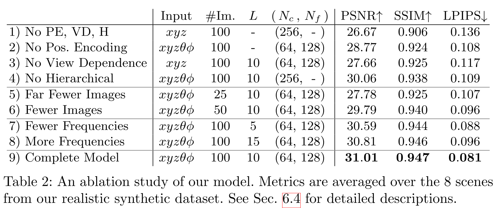
Hierarchical Volume Sampling
Our rendering strategy of densely evaluating the neural radiance field network at N query points along each camera ray is inefficient: free space and occluded regions that do not contribute to the rendered image are still sampled repeatedly. Instead of just using a single network to represent the scene, we simultaneously optimize two networks: one “coarse” and one “fine”. We first sample a set of \(N_c\) locations using stratified sampling, and evaluate the “coarse” network at these locations as described in Eqns. 2 and 3. Given the output of this “coarse” network, we then produce a more informed sampling of points along each ray where samples are biased towards the relevant parts of the volume.
At each optimization iteration, we randomly sample a batch of camera rays from the set of all pixels in the dataset, and then follow the hierarchical sampling described in Sec. 5.2 to query \(N_c\) samples from the coarse network and \(N_c + N_f\) samples from the fine network. Our loss is simply the total squared error between the rendered and true pixel colors for both the coarse and fine renderings:
\[\ell=\sum_{r\in\mathcal{R}}{\left[\lVert \hat{C}_c(r)-C(r)\rVert+\lVert \hat{C}_f(r)-C(r)\rVert\right]}\]Compared with Differential Rendering
One popular class of approaches uses mesh-based representations of scenes with either diffuse [48] or view-dependent [2,8,49] appearance. Differentiable rasterizers [4,10,23,25] or pathtracers [22,30] can directly optimize mesh representations to reproduce a set of input images using gradient descent. However, gradient-based mesh optimization based on image reprojection is often difficult, likely because of local minima or poor conditioning of the loss land- scape. Furthermore, this strategy requires a template mesh with fixed topology to be provided as an initialization before optimization [22], which is typically unavailable for unconstrained real-world scenes.
Results
Some results from bmild/nerf:
Next Steps
Cool, everything sounds great. Why we not use it to replace existing rendering method. While it is too slow. Optimizing a NeRF takes between a few hours and a day or two (depending on resolution) and only requires a single GPU. Rendering an image from an optimized NeRF takes somewhere between less than a second and ~30 seconds, again depending on resolution. But using current mesh + texture way, it won’t takes you more than few millisecond. There have been a lot of efforts made to improve the speed, which could be covered in future posts.