3D Gaussian Splatting for Real-Time Radiance Field Rendering
[face 3d-gaussian tracking dynamic nerf deep-learning This is my reading note on 3D Gaussian Splatting for Real-Time Radiance Field Rendering(best paper of SIGGRAPH 2023) and its extension Dynamic 3D Gaussians: Tracking by Persistent Dynamic View Synthesis, which enables it to track dynamic objects/scenes.
3D Gaussian Splatting achieves real-time rendering of radiance fields with quality that equals the previous method with the best quality (p. 1). Key to this performance is a novel 3D Gaussian scene representation coupled with a real-time differentiable renderer, which offers significant speedup to both scene optimization and novel view synthesis. (p. 1)
Introduction
First, starting from sparse points produced during camera calibration, we represent the scene with 3D Gaussians that preserve desirable properties of continuous volumetric radiance fields for scene optimization while avoiding unnecessary computation in empty space; Second, we perform interleaved optimization/density control of the 3D Gaussians, notably optimizing anisotropic covariance to achieve an accurate representation of the scene; Third, we develop a fast visibility-aware rendering algorithm that supports anisotropic splatting and both accelerates training and allows realtime rendering. (p. 1)
We introduce a new approach that combines the best of both worlds: our 3D Gaussian representation allows optimization with state-of-the-art (SOTA) visual quality and competitive training times, while our tile-based splatting solution ensures real-time rendering at SOTA quality for 1080p resolution on several previously published datasets (p. 1)
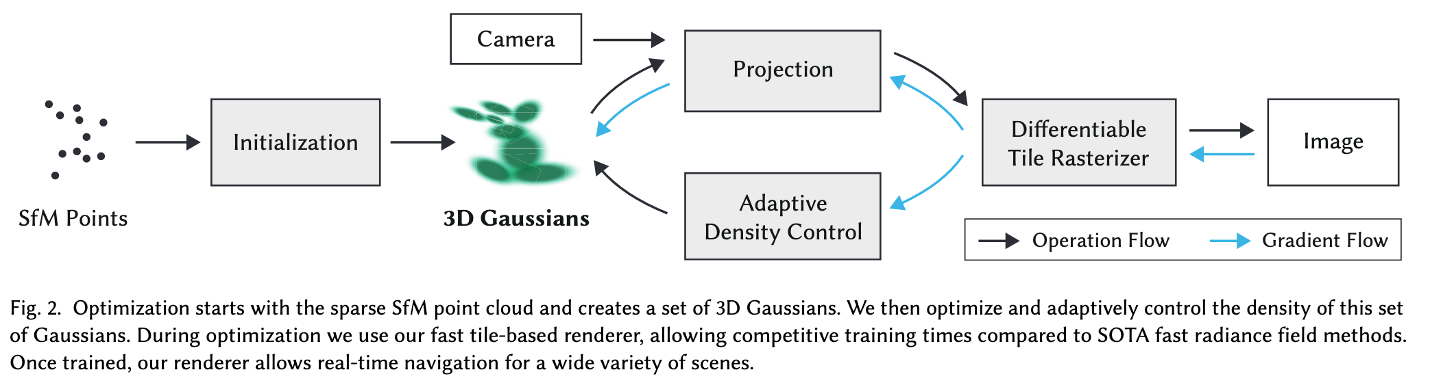
We first introduce 3D Gaussians as a flexible and expressive scene representation. We start with the same input as previous NeRF-like methods, i.e., cameras calibrated with Structure-from-Motion (SfM) [Snavely et al. 2006] and initialize the set of 3D Gaussians with the sparse point cloud produced for free as part of the SfM process. (p. 2)
We show that 3D Gaussians are an excellent choice, since they are a differentiable volumetric representation, but they can also be rasterized very efficiently by projecting them to 2D, and applying standard 𝛼-blending, using an equivalent image formation model as NeRF. The second component of our method is optimization of the properties of the 3D Gaussians – 3D position, opacity 𝛼, anisotropic covariance, and spherical harmonic (SH) coefficients – interleaved with adaptive density control steps, where we add and occasionally remove 3D Gaussians during optimization. The optimization procedure produces a reasonably compact, unstructured, and precise representation of the scene (1-5 million Gaussians for all scenes tested). The third and final element of our method is our real-time rendering solution that uses fast GPU sorting algorithms and is inspired by tile-based rasterization (p. 2)
Related Work
Neural Rendering and Radiance Fields
Most notable of these methods are InstantNGP [Müller et al. 2022] which uses a hash grid and an occupancy grid to accelerate computation and a smaller MLP to represent density and appearance; and Plenoxels [Fridovich-Keil and Yu et al. 2022] that use a sparse voxel grid to interpolate a continuous density field, and are able to forgo neural networks altogether. Both rely on Spherical Harmonics: the former to represent directional effects directly, the latter to encode its inputs to the color network. (p. 3)
Point-Based Rendering and Radiance Fields
While true to the underlying data, point sample rendering suffers from holes, causes aliasing, and is strictly discontinuous. Seminal work on high-quality point-based rendering addresses these issues by “splatting” point primitives with an extent larger than a pixel, e.g., circular or elliptic discs, ellipsoids, or surfels [Botsch et al. 2005; Pfister et al. 2000; Ren et al. 2002; Zwicker et al. 2001b]. (p. 3)
A typical neural point-based approach (e.g., [Kopanas et al. 2022, 2021]) computes the color 𝐶 of a pixel by blending N ordered points overlapping the pixel: \(C=\sum_{i\in N}{c_i \alpha_i \prod_{j=1}^{i-1}{1-\alpha_j}}\)
However, the rendering algorithm is very different. NeRFs are a continuous representation implicitly representing empty/occupied space; expensive random sampling is required to find the samples in Eq. 2 with consequent noise and computational expense. In contrast, points are an unstructured, discrete representation that is flexible enough to allow creation, destruction, and displacement of geometry similar to NeRF. (p. 3)
Our rasterization respects visibility order in contrast to their order-independent method. In addition, we backpropagate gradients on all splats in a pixel and rasterize anisotropic splats. (p. 3)
While focusing on specular effects, the diffuse point-based rendering track of Neural Point Catacaustics [Kopanas et al. 2022] overcomes this temporal instability by using an MLP, but still required MVS geometry as input (p. 3)
A recent approach [Xu et al. 2022] uses points to represent a radiance field with a radial basis function approach. They employ point pruning and densification techniques during optimization, but use volumetric ray-marching and cannot achieve real-time display rates. (p. 4)
Proposed Method
From these points we create a set of 3D Gaussians (Sec. 4), defined by a position (mean), covariance matrix and opacity 𝛼 (p. 4) The directional appearance component (color) of the radiance field is represented via spherical harmonics (SH) (p. 4)
DIFFERENTIABLE 3D GAUSSIAN SPLATTING
Our algorithm proceeds to create the radiance field representation (Sec. 5) via a sequence of optimization steps of 3D Gaussian parameters, i.e., position, covariance, 𝛼 and SH coefficients interleaved with operations for adaptive control of the Gaussian density. The key to the efficiency of our method is our tile-based rasterizer (Sec. 6) that allows 𝛼-blending of anisotropic splats, respecting visibility order thanks to fast sorting. (p. 4)
Our representation has similarities to previous methods that use 2D points [Kopanas et al. 2021; Yifan et al. 2019] and assume each point is a small planar circle with a normal (p. 4). we model the geometry as a set of 3D Gaussians that do not require normals. Our Gaussians are defined by a full 3D covariance matrix $\Sigma$ defined in world space [Zwicker et al. 2001a] centered at point (mean) $\mu$ (p. 4)
Given a viewing transformation 𝑊 the covariance matrix Σ′ in camera coordinates is given as follows: $\Sigma’=JW\Sigma W^T J^T$(5) where 𝐽 is the Jacobian of the affine approximation of the projective transformation. (p. 4)
Given a scaling matrix 𝑆 and rotation matrix 𝑅, we can find the corresponding $\Sigma=RSS^TR^T$ (p. 4). To allow independent optimization of both factors, we store them separately: a 3D vector 𝑠 for scaling and a quaternion 𝑞 to represent rotation. (p. 4). To avoid significant overhead due to automatic differentiation during training, we derive the gradients for all parameters explicitly. (p. 4)
OPTIMIZATION WITH ADAPTIVE DENSITY CONTROL OF 3D GAUSSIANS
The optimization of these parameters is interleaved with steps that control the density of the Gaussians to better represent the scene. (p. 4)

 Our optimization thus needs to be able to create geometry and also destroy or move geometry if it has been incorrectly positioned. (p. 5). We estimate the initial covariance matrix as an isotropic Gaussian with axes equal to the mean of the distance to the closest three points. (p. 5)
After optimization warm-up (see Sec. 7.1), we densify every 100 iterations and remove any Gaussians that are essentially transparent, i.e., with 𝛼 less than a threshold 𝜖𝛼 . (p. 5)
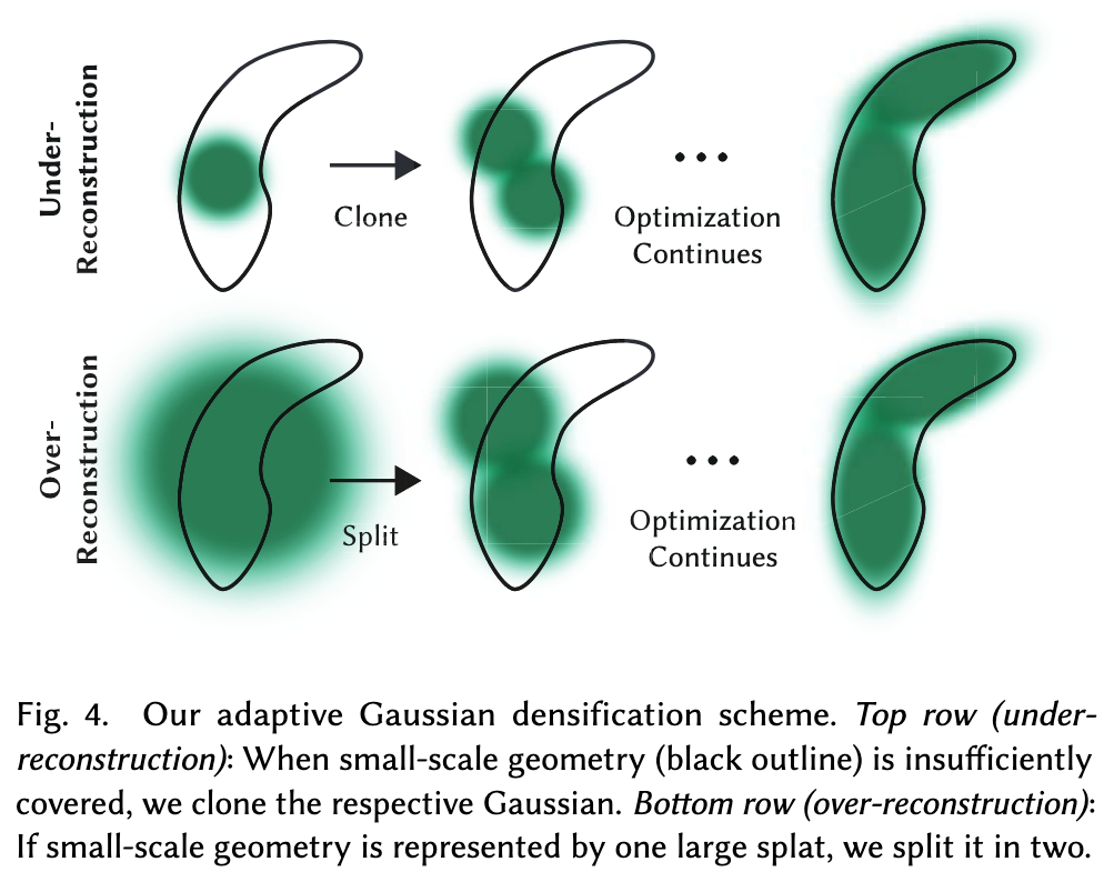
It focuses on regions with missing geometric features (“underreconstruction”), but also in regions where Gaussians cover large areas in the scene (which often correspond to “over-reconstruction”). We observe that both have large view-space positional gradients. Intuitively, this is likely because they correspond to regions that are not yet well reconstructed, and the optimization tries to move the Gaussians to correct this. (p. 5)
For small Gaussians that are in under-reconstructed regions, we need to cover the new geometry that must be created. For this, it is preferable to clone the Gaussians, by simply creating a copy of the same size, and moving it in the direction of the positional gradient. On the other hand, large Gaussians in regions with high variance need to be split into smaller Gaussians. We replace such Gaussians by two new ones, and divide their scale by a factor of 𝜙 = 1.6 which we determined experimentally. We also initialize their position by using the original 3D Gaussian as a PDF for sampling. (p. 5)

FAST DIFFERENTIABLE RASTERIZER FOR GAUSSIANS
To achieve these goals, we design a tile-based rasterizer for Gaussian splats inspired by recent software rasterization approaches [Lassner and Zollhofer 2021] to pre-sort primitives for an entire image at a time, (p. 6)
Our method starts by splitting the screen into 16×16 tiles, and then proceeds to cull 3D Gaussians against the view frustum and each tile. Specifically, we only keep Gaussians with a 99% confidence interval intersecting the view frustum. Additionally, we use a guard band to trivially reject Gaussians at extreme positions (i.e., those with means close to the near plane and far outside the view frustum), (p. 6)
After sorting Gaussians, we produce a list for each tile by identifying the first and last depth-sorted entry that splats to a given tile. For rasterization, we launch one thread block for each tile. Each block first collaboratively loads packets of Gaussians into shared memory and then, for a given pixel, accumulates color and 𝛼 values by traversing the lists front-to-back, thus maximizing the gain in parallelism both for data loading/sharing and processing. When we reach a target saturation of 𝛼 in a pixel, the corresponding thread stops. (p. 6) During rasterization, the saturation of 𝛼 is the only stopping criterion. (p. 6)
Ablation
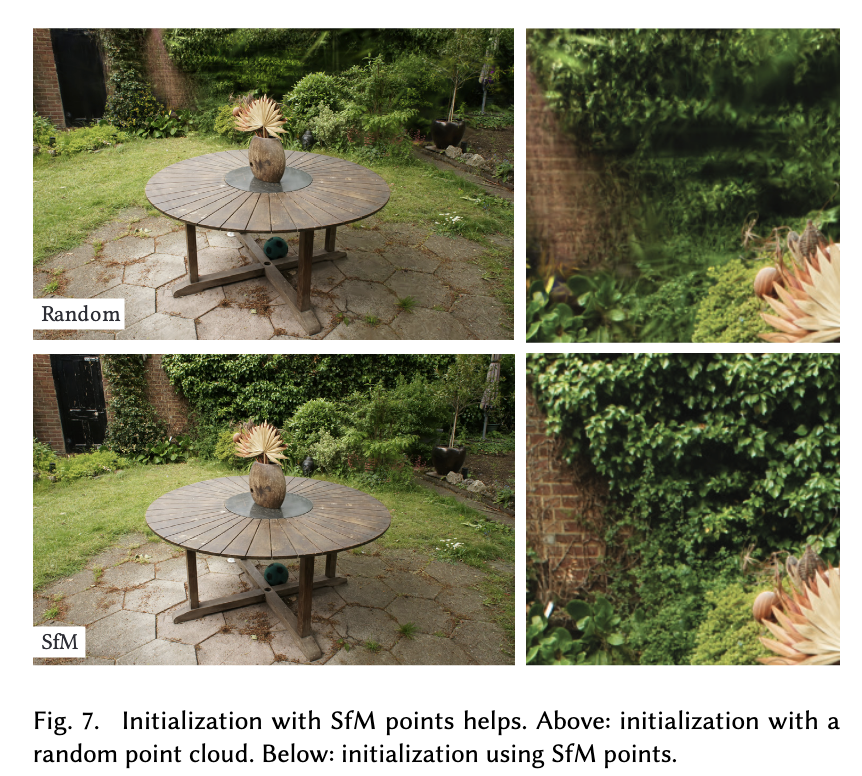
Initialization from SfM. We also assess the importance of initializ-ing the 3D Gaussians from the SfM point cloud. For this ablation, weuniformly sample a cube with a size equal to three times the extentof the input camera’s bounding box. We observe that our methodperforms relatively well, avoiding complete failure even without theSfM points. Instead, it degrades mainly in the background, see Fig. 7.Also in areas not well covered from training views, the randominitialization method appears to have more floaters that cannot beremoved by optimization. On the other hand, the synthetic NeRFdataset does not have this behavior because it has no backgroundand is well constrained by the input cameras (see discussion above).
Densification. We next evaluate our two densification methods,more specifically the clone and split strategy described in Sec. 5.We disable each method separately and optimize using the rest ofthe method unchanged. Results show that splitting big Gaussiansis important to allow good reconstruction of the background asseen in Fig. 8, while cloning the small Gaussians instead of splittingthem allows for a better and faster convergence especially whenthin structures appear in the scene.
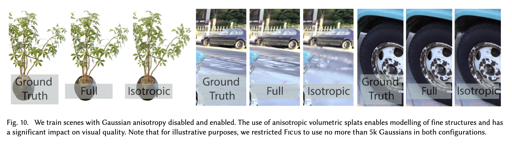
Anisotropic Covariance. An important algorithmic choice in our method is the optimization of the full covariance matrix for the 3D Gaussians. To demonstrate the effect of this choice, we perform an ablation where we remove anisotropy by optimizing a single scalar value that controls the radius of the 3D Gaussian on all three axes.The results of this optimization are presented visually in Fig. 10. We observe that the anisotropy significantly improves the quality of the 3D Gaussian’s ability to align with surfaces, which in turn allows for much higher rendering quality while maintaining the same number of points.Spherical Harmonics.
Finally, the use of spherical harmonics improves our overall PSNR scores since they compensate for the view-dependent effects (Table 3).
Limitation
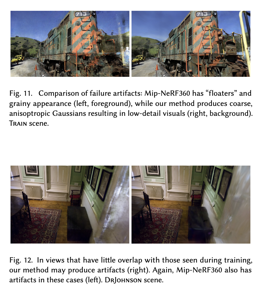
Our method is not without limitations. In regions where the sceneis not well observed we have artifacts; in such regions, other meth-ods also struggle (e.g., Mip-NeRF360 in Fig. 11). Even though theanisotropic Gaussians have many advantages as described above, our method can create elongated artifacts or “splotchy” Gaussians(see Fig. 12); again previous methods also struggle in these cases.
We also occasionally have popping artifacts when our optimization creates large Gaussians; this tends to happen in regions with view-dependent appearance. One reason for these popping artifactsis the trivial rejection of Gaussians via a guard band in the rasterizer.A more principled culling approach would alleviate these artifacts.Another factor is our simple visibility algorithm, which can lead to Gaussians suddenly switching depth/blending order. This could be addressed by antialiasing, which we leave as future work. Also, we currently do not apply any regularization to our optimization; doingso would help with both the unseen region and popping artifacts.
While we used the same hyperparameters for our full evaluation, early experiments show that reducing the position learning rate canbe necessary to converge in very large scenes.
Even though we are very compact compared to previous point-based approaches, our memory consumption is significantly higherthan NeRF-based solutions. During training of large scenes, peakGPU memory consumption can exceed 20 GB in our unoptimizedprototype. However, this figure could be significantly reduced by acareful low-level implementation of the optimization logic (similarto InstantNGP). Rendering the trained scene requires sufficient GPUmemory to store the full model (several hundred megabytes forlarge-scale scenes) and an additional 30–500 MB for the rasterizer,depending on scene size and image resolution.
Dynamic 3D Gaussians: Tracking by Persistent Dynamic View Synthesis
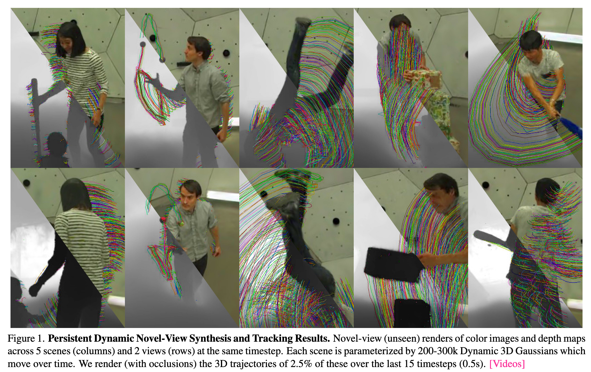 We follow an analysis-by-synthesis framework, inspired by recent work that models scenes as a collection of 3D Gaussians which are optimized to reconstruct input images via differentiable rendering. To model dynamic scenes, we allow Gaussians to move and rotate over time while enforcing that they have persistent color, opacity, and size. By regularizing Gaussians’ motion and rotation with local-rigidity constraints, we show that our Dynamic 3D Gaussians correctly model the same area of physical space over time, including the rotation of that space.
Our key insight is that we restrict all attributes of the Gaussians (such as their number, color, opacity, and size) to be the same over time, but let their position and orientation vary. This allows our Gaussians to be thought of as a particle-based physical model of the world, where oriented particles undergo rigid-body transformations over time. (p. 2)
Crucially, particles allow us to operationalize physical priors over their movement that act as regularizers for the optimization: a local rigidity prior, a local rotational-similarity prior, and a long-term local isometry prior. These priors ensure that local neighborhoods of particles move approximately rigidly between time steps, and that nearby particles remain close by over all time steps. (p. 2)
Previous approaches to neural reconstruction of dynamic scenes can be seen as either Eulerian representations that keep track of scene motion at fixed grid locations [5, 10, 36] or Lagrangian representations where an observer follows a particular particle through space and time. We fall in the latter category, but in contrast to prior point-based representations [1, 45], we make use of oriented particles that allow for richer physical priors (as above) and that directly reconstruct the 6-DOF motion of all 3D points, enabling a variety of downstream applications (see Fig. 3 and 7). (p. 2)
An remarkable feature of our approach is that tracking arises exclusively from the process of rendering per-frame images (p. 2)
Related Work
Some existing ways ore representing 3D scenes:
- Methods that represent the 3D scene in a canonical timestep and use a deformation field to warp this to the rest of the timesteps (p. 2)
- Template guided methods [13, 20, 42], which model dynamic scenes in restricted environments where the mo- tion can be modelled by a predefined template e.g. a set of human-pose skeleton transformations (p. 3)
- Point-based methods [1, 45], which compared to all of the above categories, hold the most promise for representing dynamic scenes in a way where accurate correspondence over time can emerge due to their natural Lagrangian repre- sentation. (p. 3)
Other than rendering accuracy and speed, modeling the dy- namic world with Gaussians has a distinct advantage over points as Gaussian’s have a notion of ‘rotation’ so we can use them to model the full 6 degree-of-freedom (DOF) mo- tion of a scene at every point and can use this to construct physically-plausible local rigidity losses. (p. 3)
The most similar method to ours is OmniMotion [40] which also fits a dynamic radiance field representation using test-time optimization for the purpose of long-term track- ing. They focus on monocular video while we focus on multi-camera capture and as such we can reconstruct tracks in metric-3D while they produce a ‘pseudo-3D’ representa- tion (p. 3)
Proposed Method
The reconstruction is performed temporally online, i.e., one timestep of the scene is reconstructed at a time with each one being initialized using the previous timestep’s representation. The first timestep acts as an initialization for our scene where we optimize all properties, and then fix all for the subsequent timesteps except those defining the motion of the scene. Each timestep is trained via gradient based optimization using a differentiable renderer (R) to render the scene at each timestep into each of the training cameras. \(\hat{I}_{t,c} = R(S_t, K_c, E_{t,c})\)
Our dynamic scene representation (S) is parameterized by a set of Dynamic 3D Gaussians, each of which has the following parameters:
- a 3D center for each timestep $(x_t, y_t, z_t)$.
- a 3D rotation for each timestep parameterized by a quaternion $(qw_t, qx_t, qy_t, qz_t)$.
- a 3D size in standard deviations (consistent over all timesteps) $(s_x, s_y, s_z)$
- a color (consistent over all timesteps) (r, g, b)
- an opacity logit (consistent over all timesteps) (o)
- a background logit (consistent over timesteps) (bg) (p. 4)
In our experiments, scenes are represented by between 200- 300k Gaussians, of which only 30-100k usually are not part of the static background. While the code contains the ability to represent view-dependent color using spherical harmon- ics, we turn this off in our experiments for simplicity. (p. 4)
The softness of this Gaussian representation also means that Gaussians typically need to significantly overlap in order to represent a physically solid object. (p. 4)
The center of the Gaussian is splatted using the standard point rendering formula: $µ^{2D} = K\frac{E_\mu}{(E_\mu)_z}$ where the 3D Gaussian center µ is projected into a 2D im- age by multiplication with the world-to-camera extrinsic matrix E, z-normalization, and multiplication by the intrin- sic projection matrix K (p. 4)
The influence of all Gaussians on this pixel can be combined by sorting the Gaussians in depth order and performing front-to-back volume rendering using the Max [24] volume rendering formula (the same as is used in NeRF [25]): \(C_{pix}=\sum_{i\in S}{c_i f_{i,pix}^{2D}\prod_{j=1}^{i-1}{1-f_{i,pix}^{2D}}}\)
Physic Prior for Tracking
We find that just fixing the color, opacity and size of Gaussians is not enough on its own to generate long-term persistent tracks, especially across ar- eas of the scene where there is a large area of near uni- form colour. In such situation the Gaussians move freely around the area of similar colour as there is no restriction on them doing so (p. 5)
We introduce three regularization losses, short-term local-rigidity Lrigid and local-rotation similarity Lrot losses and a long-term local-isometry loss. The most important of these is the local-rigidity loss , defined as: \(L_{i,j}^{rigid}=w_{i,j}\lVert (\mu_{j,t-1}-\mu_{i,t-1})-R_{i,t-1}R_{i,t}^{-1}(\mu_{j,t}-\mu_{i,t})\rVert_2\) \(L^{rigid}=\frac{1}{k\lvert S\rvert}\sum_{i\in S}\sum_{j\in knn_i}L_{i,j}^{rigid}\) This states that, for each Gaussian i, nearby Gaussians j should move in a way that follows the rigid-body transform of the coordinate system of i between timesteps. See (p. 5)
We restrict the set of Gaussians j to be the k-nearest- neighbours of i (k=20), and weight the loss by the a weight- ing factor for the Gaussian pair: \(w_{i,j}=e^{-\lambda_w\lVert \mu_{j,0}-\mu_{i,0}\rVert_2^2}\)
however we found better convergence if we explicitly force neighbouring Gaussians to have the same rotation over time: \(L^{rot}=\frac{1}{k\lvert S\rvert}\sum_{i\in S}\sum_{j\in knn_i}w_{i,j}\lVert \hat{q}_{j,t}\hat{q}_{j,t-1}^{-1}-\hat{q}_{i,t}\hat{q}_{i,t-1}^{-1}\rVert_2\) We apply $L^{rigid}$ and $L^{rot}$ only between the current timestep and the directly preceding timestep, thus only enforcing these losses over short-time horizons. Which sometimes causes elements of the scene to drift apart, thus we apply a third loss, the isometry loss, over the long-term: \(L^{iso}=\frac{1}{k\lvert S\rvert}\sum_{i\in S}\sum_{j\in knn_i}w_{i,j}\lvert\lVert \mu_{j,0}-\mu_{i,0}\rVert_2-\lVert \mu_{j,t}-\mu_{i,t}\rVert_2\rvert\)
forcing the positions between two Gaussians to be the same it only enforces the distances between them to be the same. (p. 6)
In the first timestep we initialize the scene using a coarse point cloud that could be obtained from running colmap, but instead we use available sparse samples from depth cameras. Note that these depth values are only used for initializing a sparse point cloud in the first timestep and are not used at all during optimization. We use the densification from [17] in the first timestep in order to increase the density of Gaussians and achieve a high quality reconstruction (p. 6)
We noticed that often the shirt was being mis-tracked as it was confused with the back- ground, while more contrastive elements like pants and hair were being tracked correctly. (p. 6)
To determine the correspondence of any point in 3D space p across timesteps, we can linearize the motion- space by simply taking the point’s location in the coordinate system of the Gaussian that has the most influence f(p) over this point (or the static background coordinate system if f(p) < 0.5 for all Gaussians) (p. 6)