Search Images with Image
[cbir vision image-search content-based-image-retrival If you use Google Images Search, you may find you are allowed to search images with image (uploading it or providing the url of the image). The returned results are visually similar to the query image.
Based on 以图搜图技术演进和架构优化
Overview
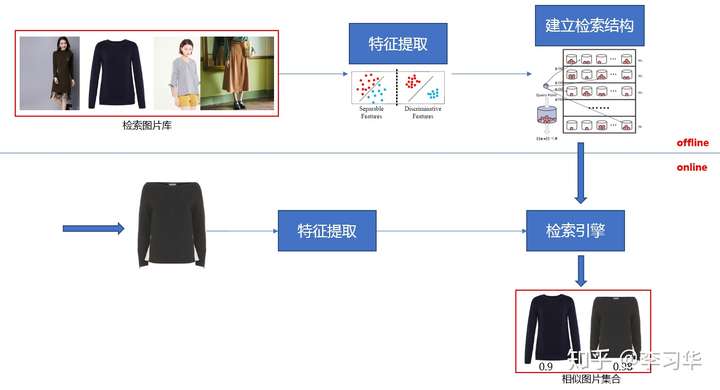
The typical system contains an offline stage, which builds up the database, and an online stage, which extracts feature from the query and query the database.
The offline stage contains the following steps:
- image database
- feature extraction, e.g., histogram (of color, gradient), bag of words, semantic feature
- indexing, e.g., KD-tree, locallity sensitive hash (LSH)
In the sections below, we will describe the details of each aspects.
Feature
Traditional Feature
There are many features proposed for image query, e.g., histogram (of color), histogram of gradient (HoG), Scale Invarient Feature Transform (SIFT), Speeded Up Robust Feature (SURF):
- HOG: for each location, gradient is computed for each pixel of nearby pixels. The gradients are then put into a histogram based on their orientation. To make the description more informative, multiple histograms are generated by dividing the neighor into 4 cells.
- SIFT: a set of keypoints are extracted from the image; for each of the keypoint, a set of orientation histograms is created on 4×4 pixel neighborhoods with 8 bins (directions) each and thus each SIFT is described as a vector of 128 dimensions.
- SURF: similar as SIFT, but wavelet response is used to compute the gradient.
Note for HOG, SIFT and SURF, the description will be normalized in order to be robust over illumination changes.
After descriptors are obtained, aggregation is then applied to merge all the descriptors of the image into a single feature vector. Several ways has been proposed, e.g.,
- Bag Of Words (BOW): a codebook is computed (e.g., k-means) from the descriptors of all images in the database, then the feature vector of an image is the assignment of its descriptors for the computed database.
- VLAD: the first step is similar to BOW. For each of the k clusters, the residuals (vector differences between descriptors and cluster centers) are accumulated, and the k 128-D sums of residuals are concatenated into a single k × 128 dimensional descriptor; we refer to it as the unnormalized VLAD.
- Fisher Vector: instead of using codebook, Fisher Vector uses the Gaussian mixture model: \(q_{ik} = \frac {\exp\left[-\frac{1}{2}(x_i - \mu_k)^T \Sigma_k^{-1} (x_i - \mu_k)\right]} {\sum_{t=1}^K \exp\left[-\frac{1}{2}(x_i - \mu_t)^T \Sigma_k^{-1} (x_i - \mu_t)\right]}\) \(\begin{align*} u_{jk} &= {1 \over {N \sqrt{\pi_k}}} \sum_{i=1}^{N} q_{ik} \frac{x_{ji} - \mu_{jk}}{\sigma_{jk}}, \\ v_{jk} &= {1 \over {N \sqrt{2 \pi_k}}} \sum_{i=1}^{N} q_{ik} \left[ \left(\frac{x_{ji} - \mu_{jk}}{\sigma_{jk}}\right)^2 - 1 \right]. \end{align*}\) then the final vector is \(\Phi(I) = \begin{bmatrix} \vdots \\ u_k \\ \vdots \\ v_k \\ \vdots \end{bmatrix}\)
Deep Learning Feature
Since the success of convolution neural network in image classification, more and more works are proposing to use the convolution neural network as the feature detector of the image, e.g., End-to-end Learning of Deep Visual Representations for Image Retrieval and Collaborative Index Embedding for Image Retrieval. Those works has suggested the top level response map (which captures semantic information) doesn’t work as well as the intemediate level response map for image retrieval. Pooling method is then applied to aggregate the response map into the feature vector, e.g.,:
- sum pooling
- max pooling
- average pooling
- MOP Pooling (Multi-scale Orderless Pooling): Our proposed feature is a concatenation of the feature vectors from three levels: (a)Level 1, corresponding to the 4096-dimensional CNN activation for the entire 256x256image; (b) Level 2, formed by extracting activations from 128x128 patches and VLADpooling them with a codebook of 100 centers; (c) Level 3, formed in the same way aslevel 2 but with 64*64 patches.
- Cross dimensional weighted pooling: each feature channels receive its own weight based on its importance to image retrieval.
- RMAC pooling: similar as MOP Pooling, but the pooling happens on the response map instead of the input.
Typically the network is finetuned for improving the performance on the image retrieval:
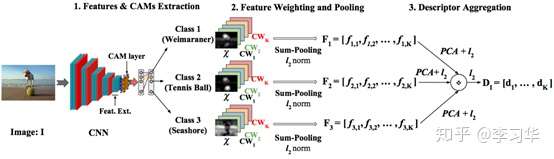
- Class weighted conv features
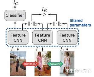
- Combining category loss and triplet loss:
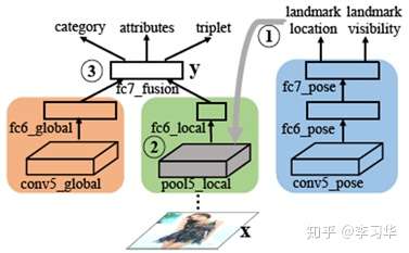
- Multi-task
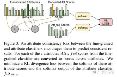
- KL-divergence
Indexing
KD-tree is an classical method for indexing multi-dimensional feature vectors. For modern system, (locallity sensitive) hash and productivity quantization is widely used.
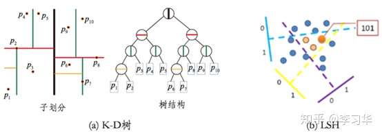
KD-tree
In a nutshell, KD-tree partition the high dimensional space by halves at each step, according to one of the feature dimension and then repeat this step until certain criterion. kd-trees are not suitable for efficiently finding the nearest neighbour in high dimensional spaces. In very high dimensional spaces, the curse of dimensionality causes the algorithm to need to visit many more branches than in lower dimensional spaces.
Locality Sensitive Hash
LSH is a way to randomly partition the ambient space into cells that respect the desired similarity metric. The core building block of LSH are locality-sensitive hash functions. We say that a hash function (or more precisely, a family of hash functions) is locality sensitive if the following property holds: pairs of points that are close together are more likely to collide than pairs of points that are far apart. LSH data structures use locality-sensitive hash functions in order to partition the space in wich the dataset lives: every possible hash value essentially corresponds to its own cell.
Productivity Quantization (PQ)
Product quantization (PQ) is an effective vector quantization method. A product quantizer can generate an exponentially large codebook at very low memory/time cost. The essence of PQ is to decompose the high-dimensional vector space into the Cartesian product of subspaces and then quantize these subspaces separately.