CLIP Learning Transferable Visual Models From Natural Language Supervision
[multimodality zero-shot clip deep-learning resnet imagenet transformer unsupervised-learning This my reading note on Learning Transferable Visual Models From Natural Language Supervision. The proposed method is called Contrastive Language-Image Pre-training or CLIP. State-of-the-art computer vision systems are trained to predict a fixed set of predetermined object categories. We demonstrate that the simple pre-training task of predicting which caption (freeform text instead of strict labeling) goes with which image is an efficient and scalable way to learn SOTA image representations from scratch on a dataset of 400 million (image, text) pairs collected from the internet. After pre-training, natural language is used to reference learned visual concepts (or describe new ones) enabling zero-shot transfer of the model to downstream tasks.
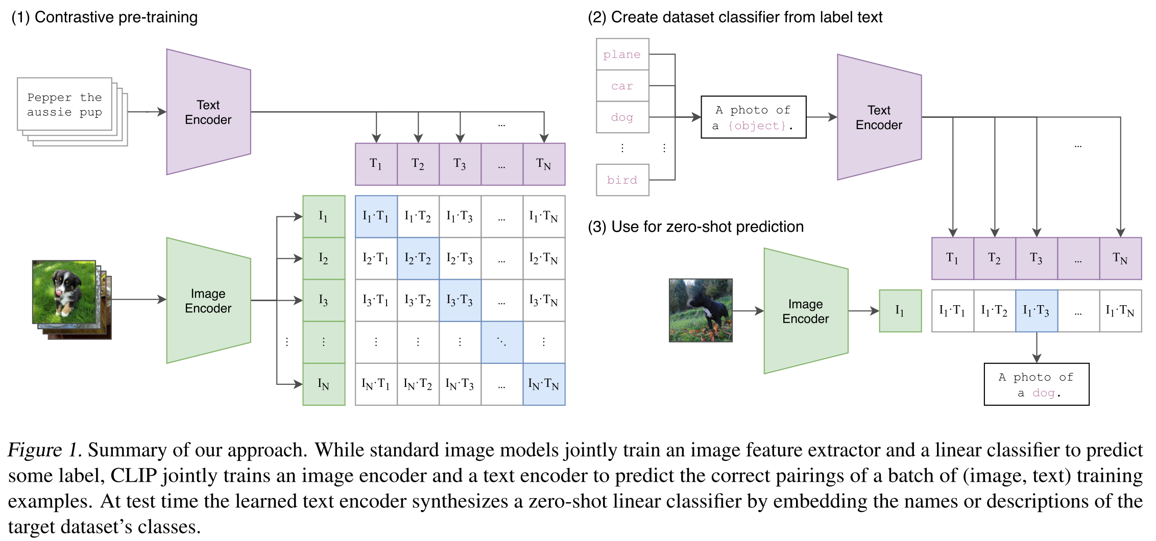
CLIP is very simple: it jointly learn an image encoder (could be CNN like ResNet or transformer like ViT) and a text encoder (transformer), such that the features of matching image and text pair are more similar than the features of unmatching image and text pair within the batch. This is described as peseudo code as below. This not only removes the requirement of strict labeling for each image in the dataset; but only the caption associated with image provides more context for the labeling.
# image_encoder - ResNet or Vision Transformer
# text_encoder - CBOW or Text Transformer
# I[n, h, w, c] - minibatch of aligned images
# T[n, l] - minibatch of aligned texts
# W_i[d_i, d_e] - learned proj of image to embed
# W_t[d_t, d_e] - learned proj of text to embed
# t - learned temperature parameter
# extract feature representations of each modality
I_f = image_encoder(I) #[n, d_i]
T_f = text_encoder(T) #[n, d_t]
# joint multimodal embedding [n, d_e]
I_e = l2_normalize(np.dot(I_f, W_i), axis=1)
T_e = l2_normalize(np.dot(T_f, W_t), axis=1)
# scaled pairwise cosine similarities [n, n]
logits = np.dot(I_e, T_e.T) * np.exp(t)
# symmetric loss function
labels = np.arange(n)
loss_i = cross_entropy_loss(logits, labels, axis=0)
loss_t = cross_entropy_loss(logits, labels, axis=1)
loss = (loss_i + loss_t)/2
To attempt to cover as broad a set of visual concepts as possible, we search for (image, text) pairs as part of the construction process whose text includes one of a set of 500,000 queries.
Encoder
Due to the large size of our pre-training dataset, over-fitting is not a major concern. We train CLIP from scratch without initializing the image encoder with ImageNet weights or the text encoder with pre-trained weights. We do not use the non-linear projection between the representation and the contrastive embedding space, a change which was introduced by Bachman et al. (2019) and popularized by Chen et al. (2020b). We instead use only a linear projection to map from each encoder’s representation to the multi-modal embedding space.
We consider two different architectures for the image encoder. For the first, we use ResNet-50 (He et al., 2016a) as the base architecture for the image encoder. We make sev- eral modifications to the original version using the ResNet- D improvements from He et al. (2019) and the antialiased rect-2 blur pooling from Zhang (2019). We also replace the global average pooling layer with an attention pooling mechanism. The attention pooling is implemented as a sin- gle layer of “transformer-style” multi-head QKV attention where the query is conditioned on the global average-pooled representation of the image. For the second architecture, we experiment with the recently introduced Vision Transformer (ViT) (Dosovitskiy
The text encoder is a Transformer. As a base size we use a 63M-parameter 12- layer 512-wide model with 8 attention heads. The trans- former operates on a lower-cased byte pair encoding (BPE) representation of the text with a 49,152 vocab size (Sen- nrich et al., 2015). For computational efficiency, the max sequence length was capped at 76. The text sequence is bracketed with [SOS] and [EOS] tokens.
Training
We train a series of 5 ResNets and 3 Vision Transformers. For the ResNets we train a ResNet-50, a ResNet-101, and then 3 more which follow EfficientNet-style model scaling and use approximately 4x, 16x, and 64x the compute of a ResNet-50. They are denoted as RN50x4, RN50x16, and RN50x64 respectively. For the Vision Transformers we train a ViT-B/32, a ViT-B/16, and a ViT-L/14. We train all models for 32 epochs. We use the Adam optimizer (Kingma & Ba, 2014) with decoupled weight decay regularization (Loshchilov & Hutter, 2017) applied to all weights that are not gains or biases, and decay the learning rate using a cosine schedule.
We use a very large minibatch size of 32,768. Mixed-precision (Micikevicius et al., 2017) was used to accelerate training and save memory. The largest ResNet model, RN50x64, took 18 days to train on 592 V100 GPUs while the largest Vision Transformer took 12 days on 256 V100 GPUs.
Experiment
CLIP is evaluated as zero-shot classifier for image classification task. For each dataset, we use the names of all the classes in the dataset as the set of potential text pairings and predict the most probable (image, text) pair according to CLIP. Then the pair with largest cosine similarity between image feature and text feature is chosen as the classification result.
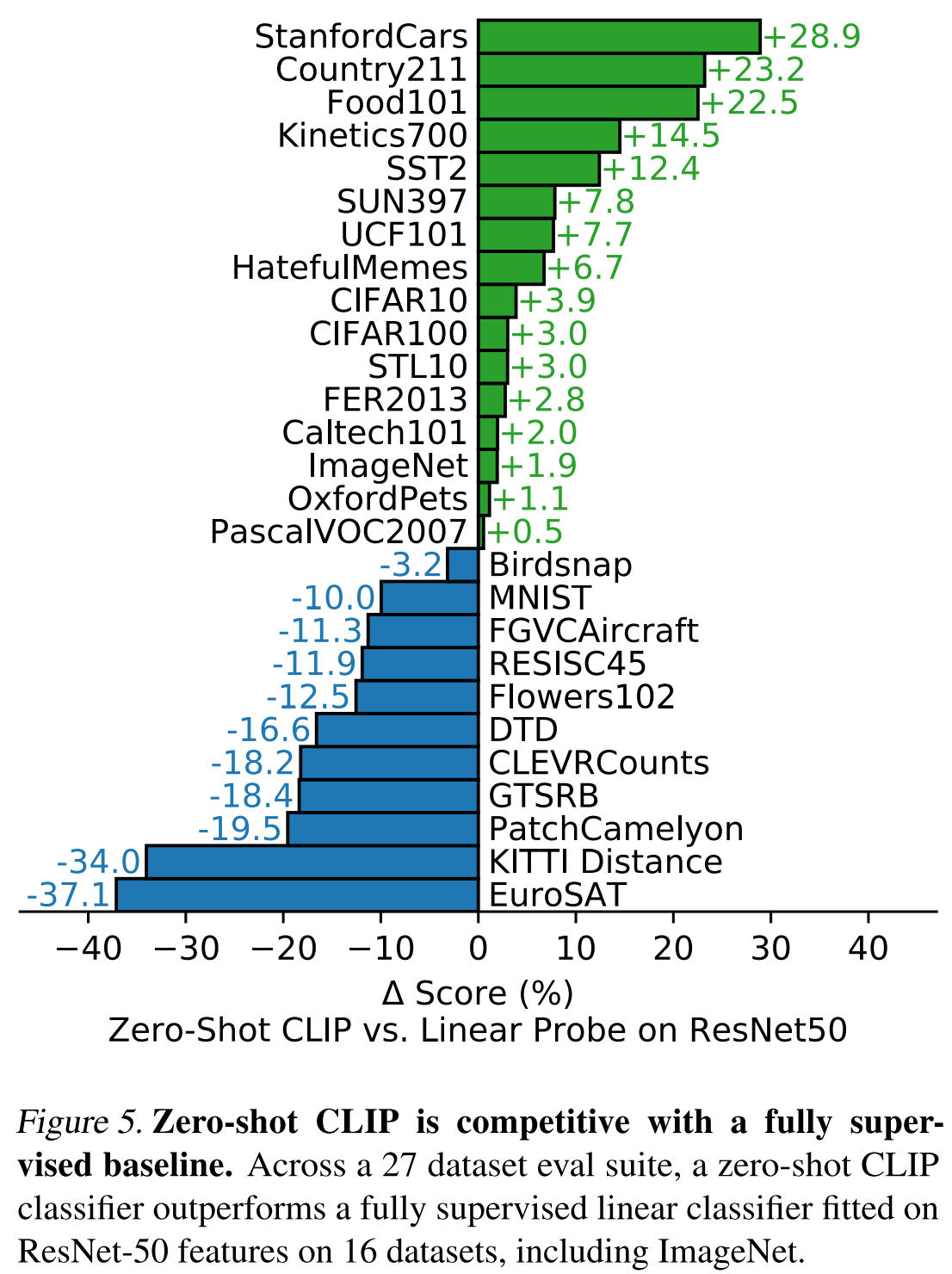
Figure 5 shows a comparison between CLIP vs supervised classifer with ResNet 50 on 27 datasets. Zero-shot CLIP outperforms this baseline slightly more often than not and wins on 16 of the 27 datasets:
- On fine-grained classification tasks, we observe a wide spread in performance. We suspect these difference are primarily due to varying amounts of per-task supervision between WIT and ImageNet.
- On “general” object classifica- tion datasets such as ImageNet, CIFAR10/100, STL10, and PascalVOC2007 performance is relatively similar with a slight advantage for zero-shot CLIP in all cases.
- Zero- shot CLIP significantly outperforms a ResNet-50 on two datasets measuring action recognition in videos.
- we see that zero-shot CLIP is quite weak on several spe- cialized, complex, or abstract tasks such as satellite image classification (EuroSAT and RESISC45), lymph node tumor detection (PatchCamelyon), counting objects in synthetic scenes (CLEVRCounts), self-driving related tasks such as German traffic sign recognition (GTSRB), recognizing distance to the nearest car (KITTI Distance). These results highlight the poor capability of zero-shot CLIP on more complex tasks.
Linear probe means training a classifier on the feature of model supervisedly.
Figure 6 compares CLIP vs few-shot methods. When comparing zero-shot CLIP to few-shot logistic regression on the features of other models, zero-shot CLIP roughly matches the performance of the best performing 16-shot classifier in our evaluation suite.
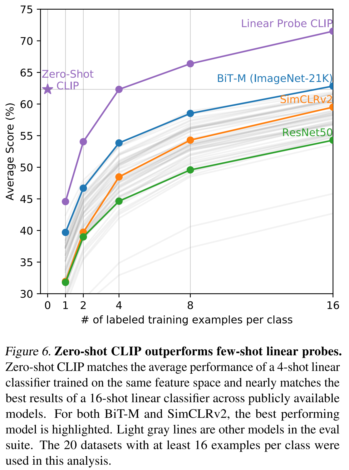
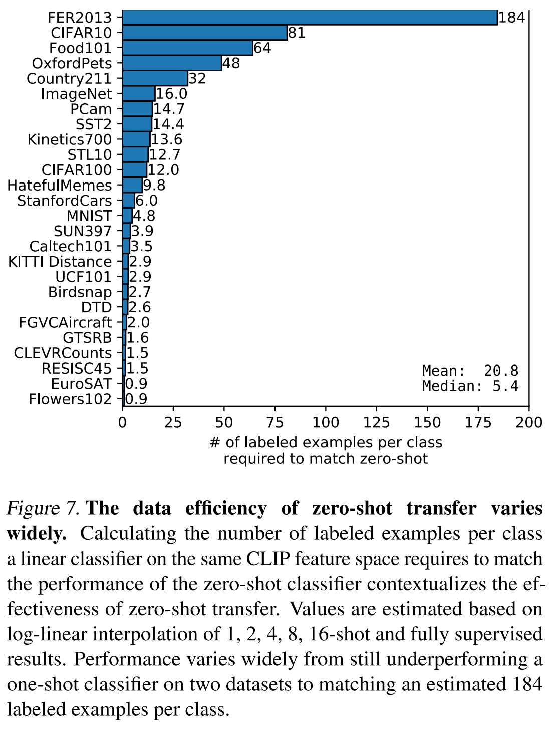
Figure 7 compares the number of labeled examples per class a linear classifier on the same CLIP feature space requires to match the performance of the zero-shot classifier contextualizes the effectiveness of zero-shot transfer.
Prompt
CLIP also found how to build the text/caption from the class labling could affect the accuracy, by upto 5% on ImageNet!. A common issue is polysemy. When the name of a class is the only information provided to CLIP’s text encoder it is unable to differentiate which word sense is meant due to the lack of context. In some cases multiple meanings of the same word might be included as different classes in the same dataset! This happens in ImageNet which contains both construction cranes and cranes that fly
To help bridge this distribution gap, we found that using the prompt template “A photo of a {label}.” to be a good default that helps specify the text is about the content of the image. This often improves performance over the baseline of using only the label text. For instance, just using this prompt improves accuracy on ImageNet by 1.3%.
We have also observed that zero-shot performance can be significantly improved by customizing the prompt text to each task. A few, non exhaustive, examples follow. We found on several fine-grained image classification datasets that it helped to specify the category. For example on Oxford-IIIT Pets, using “A photo of a {label}, a type of pet.” to help provide context worked well. Likewise,
We also experimented with ensembling over multiple zero-shot classifiers as another way of improving performance. These classifiers are computed by using different context prompts such as ‘A photo of a big {label}” and “A photo of a small {label}”. We construct the ensemble over the embedding space instead of probability space. We’ve observed ensembling across many gen- erated zero-shot classifiers to reliably improve performance and use it for the majority of datasets. On ImageNet, we ensemble 80 different context prompts and this improves performance by an additional 3.5% over the single default prompt discussed above. When considered together, prompt engineering and ensembling improve ImageNet accuracy by almost 5%.