Face Recognition
[deep-learning face Face recognition (FR) has been the prominent biometric technique for identity authentication and has been widely used in many areas, such as military, finance, public security and daily life.
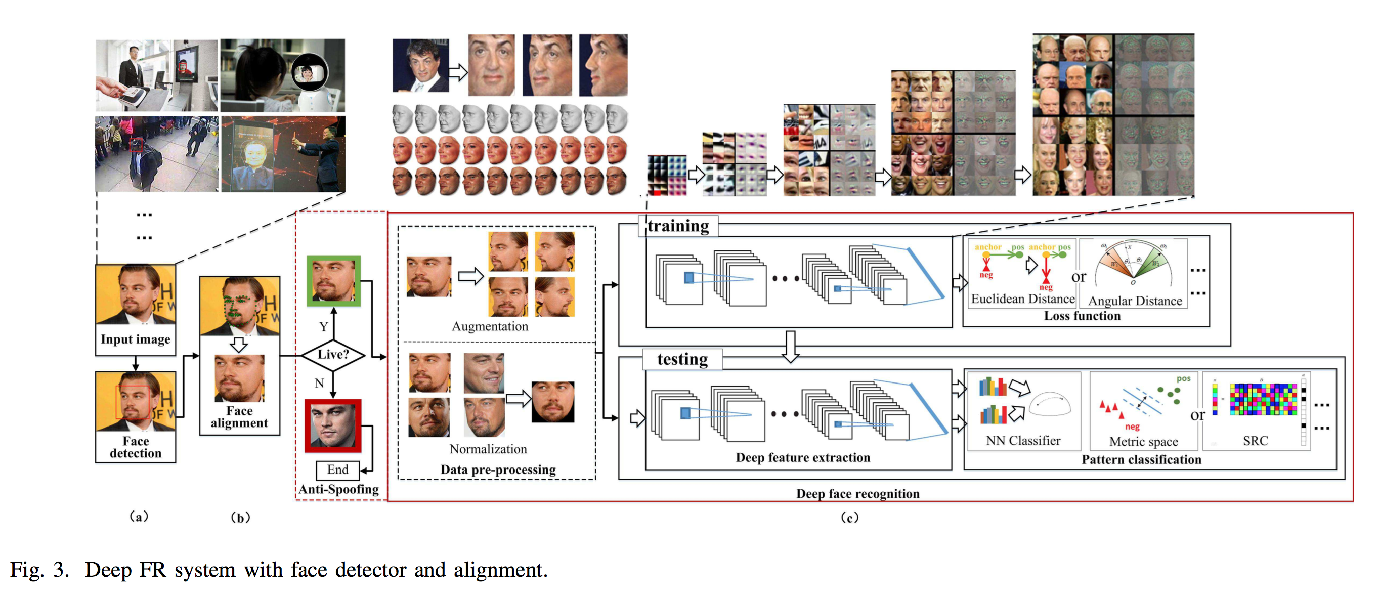
There are three modules needed for the whole system
- a face detector is used to localize faces in images or videos.
- with the facial landmark detector, the faces are aligned to normalized canonical coordinates.
- the FR module is implemented with these aligned face images.
Before a face image is fed to an FR module, face anti-spoofing, which recognizes whether the face is live or spoofed, can avoid different types of attacks.
FR can be categorized as face verification and face identification.
- Face verification computes one-to-one similarity between the gallery and probe to determine whether the two images are of the same subject
- face identification computes one-to-many similarity to determine the specific identity of a probe face.
Typical FR algorithms is consisted of some backbone and loss functions. Typically backbones includes:
- backbones used for image classification, e.g., AlexNet, VGG, GoogLeNet, ResNet
- backbone specially designed for FR, e.g., SENet
Loss Function
The softmax loss is commonly used as the supervision signal in object recognition, and it encourages the separability of features. However, for FR, when intra- variations could be larger than inter-differences, the softmax loss is not sufficiently effective for FR. The commonly used ones are described below:
- Euclidean-distance-based loss: compressing intra- variance and enlarging inter-variance based on Euclidean distance. Typically constrastive loss or triplet loss are used as the loss function. The contrastive loss
- constrastive loss requires face image pairs and then pulls together positive pairs and pushes apart negative pairs. The problem for constrastive loss is that the margin $\epsilon$ is not easy to choose \(\ell=y_{i,j}\max{(0,\lvert f(x_i) -f(x_j)\rvert_2-\epsilon)}+(1-y_{i,j})\max{(0,\epsilon-\lvert f(x_i) -f(x_j)\rvert_2)}\)
- triplet loss considers the relative difference of the distances between the absolute distances of the matching pairs and non-matching pairs \(\lvert f(x_i^a)-f(x_i^p)\rvert_2 + \epsilon < \lvert f(x_i^a) -f(x_i^n)\rvert_2\)
- center loss: enforces the differences of feature to its class center is small \(\ell_c=\sum_{i\in y_i=c}{x_i - c_{y_i}}\)
- angular/cosine-margin-based loss: learning discriminative face features in terms of angular similarity, leading to potentially larger angular/cosine separability between learned features. \(\ell_i=-\log{\frac{e^{\lvert w_{y_i}\rvert \lvert x_i\rvert \phi(\theta_{y_i})}}{e^{\lvert w_{y_i}\rvert \lvert x_i\rvert \phi(\theta_{y_i})}+\sum_{j\neq y_i}{e^{\lvert w_{y_i}\rvert \lvert x_i\rvert \cos(\theta_j)}}}}\) $\theta$ is the angle between $W$ and $x$.
- softmax loss and its variations: directly using softmax loss or modifying it to improve performance, e.g., L2 normalization on features or weights as well as noise injection.
Algorithms
DeepFace
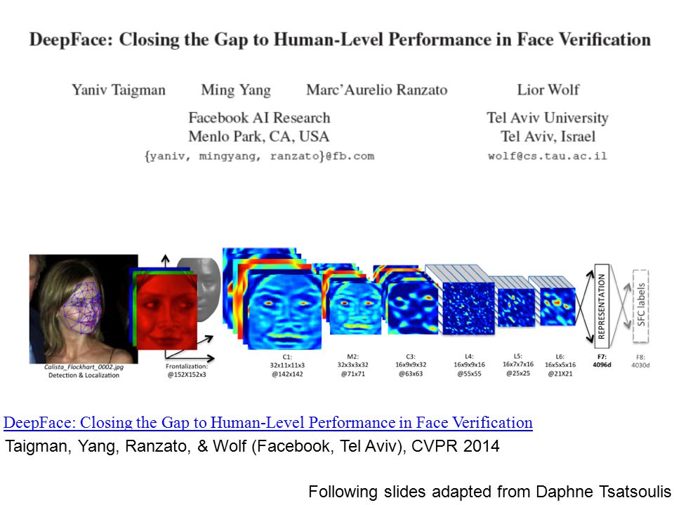
AlexNet + Softmax/Euclidean
DeepID
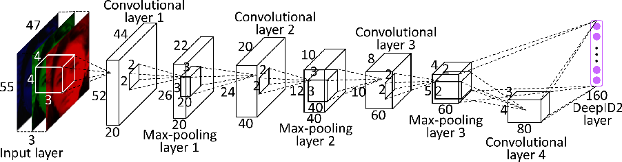
Customized neural network + Constrastive loss/Euclidean
FaceNet
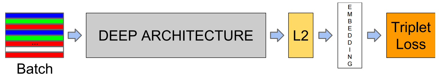
AlextNet + triplet loss/Euclidean
VGGface
VGGNet + triplet loss/Euclidean
SphereFace
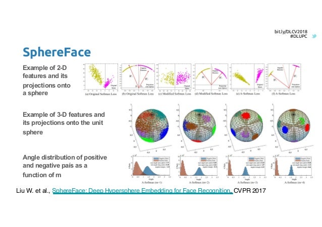
ResNet + angular loss
SEnet
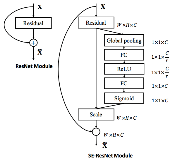
The motivation of Sequeeze and Excitation net (SEnet) is to calibrate channel-wise feature response by analyzing the interdependencies between channels.
The squeeze steps takes a response and (average) pools within each output channel (i.e., $\mathbb{R}^{H\times W\times C}\to\mathbb{R}^{1\times C}$). The excitation steps takes it as input to compute a per-channel modulation weight with bottleneck layer $F_{ex}(z, W) = \sigma(W_2\delta(W_1 z))$. The weight is then applied to the response.
In later layers, the SE blocks become increasingly specialised, and respond to different inputs in a highly class-specific manner.
Light CNN
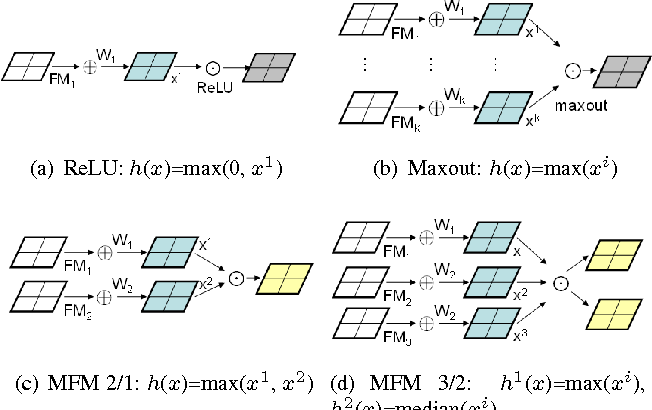
LightCNN proposes a new activation function for convolution layer: Max-Feature-Map (MFM), which could not only reject noisy label but also perform feature selection. It is motivated by the lateral inhibition in neural science, where a neuron receives high response tends to suppress neighboring or related neurons.
For example, a MFM 2/1 for a response $x\in\mathbb{R}^{H\times W\times 2N}$ can be written as:
\[\hat{x}_{i,j}^k = \max{(x_{i,j}^k, x_{i,j}^{k+N})}\]Simiarly a MFM 3/2 can be written as: \(\hat{x}_{i,j}^{k_1} = \max{(x_{i,j}^k, x_{i,j}^{k+N}, x_{i,j}^{k+2N})}\\\hat{x}_{i,j}^{k_2} = median{(x_{i,j}^k, x_{i,j}^{k+N}, x_{i,j}^{k+2N})}\)
Bilinear CNN
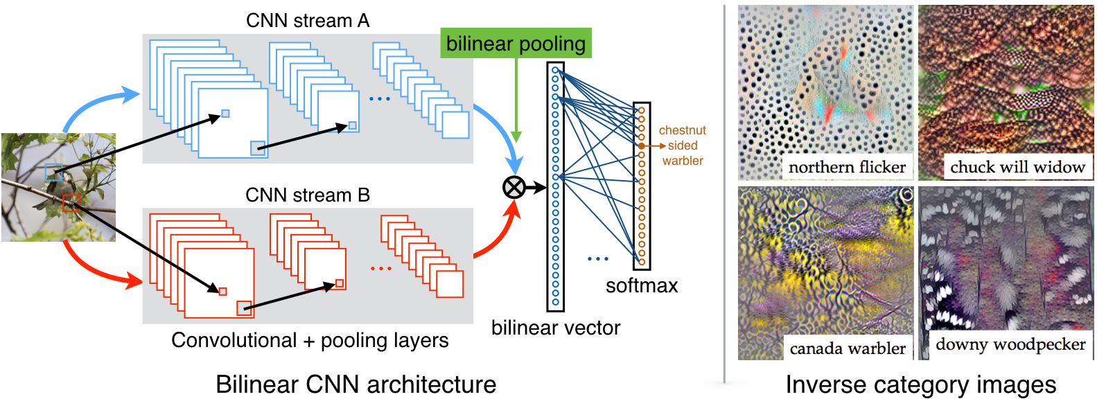
Bilinear CNN is a recognition architecture that consists of two feature extractors whose outputs are multiplied using outer product at each location of the image and pooled to obtain an image descriptor.
For example, if one extrators creates feature $x\in\mathbb{R}^{C\times M}$ and the other creates feature $y\in\mathbb{R}^{C\times N}$, the bilinear feature would be $z = x^T\times y\in\mathbb{R}^{M\times N}$. This feature is then pooled.
Pairwise Relation Network
Pairwise relational network (PRN) obtains local appearance patches around landmark points on the feature map, and captures the pairwise relation between a pair of local appearance patches.
To capture relations, the PRN takes local appearance patches as input by ROI projection around landmark points on the feature map in a backbone CNN network (ResNet). With these local appearance patches, the PRN is trained to capture unique pairwise relations between pairs of local appearance patches to determine facial part- relational structures and properties in face images.
The facial identity state feature is learned from the long short-term memory (LSTM) units network with the sequential local appearance patches on the feature maps.
MobiFace
Mobilenetv2