GIRAFFE Representing Scenes as Compositional Generative Neural Feature Fields
[graf cnn gan nerf mlp composition giraffe deep-learning differential-rendering This is my reading note for GIRAFFE: Representing Scenes as Compositional Generative Neural Feature Fields. The paper aims to provide more control to 3D object rendering NeRF. For example moving the objects in the 3D scene, adding/deleting objects and so on. To acheive this, GIRAFFE proposed to model the objects and background in the scene separately and then composite together for the rendering. In addition, different from NeRF, GIRAFFE uses a learned discriminator instead of L2 or L1 loss as loss function, thus it is a GAN.
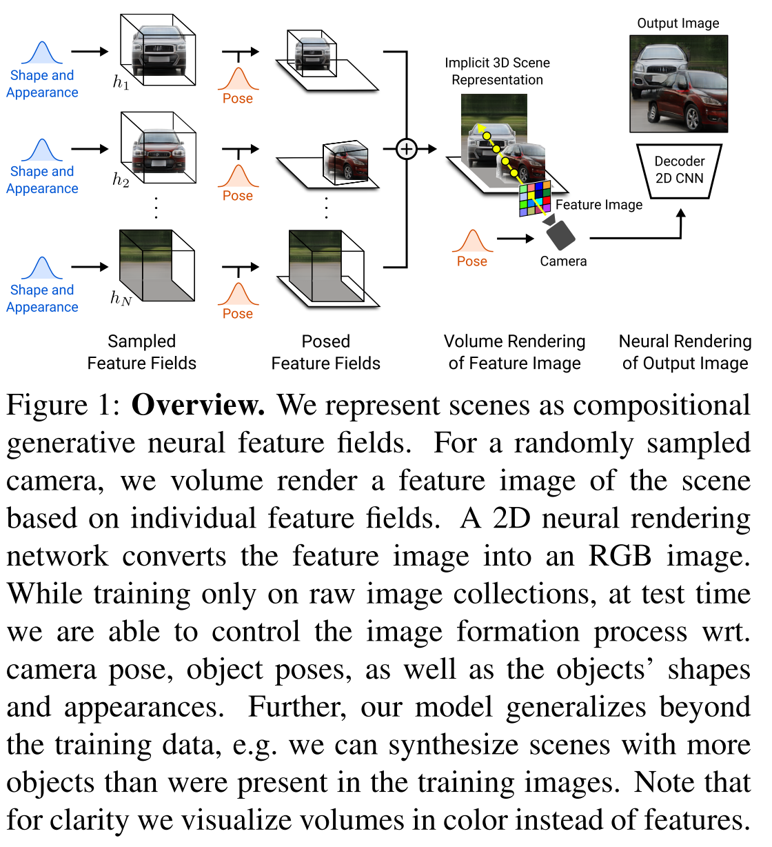
The figure below provides an over view of the algorithm. It roughly consists of three components: generator (one for each object plus one for background), scene compositor, volume render (3D to 2D) and discriminator. They will be describd with more details below.
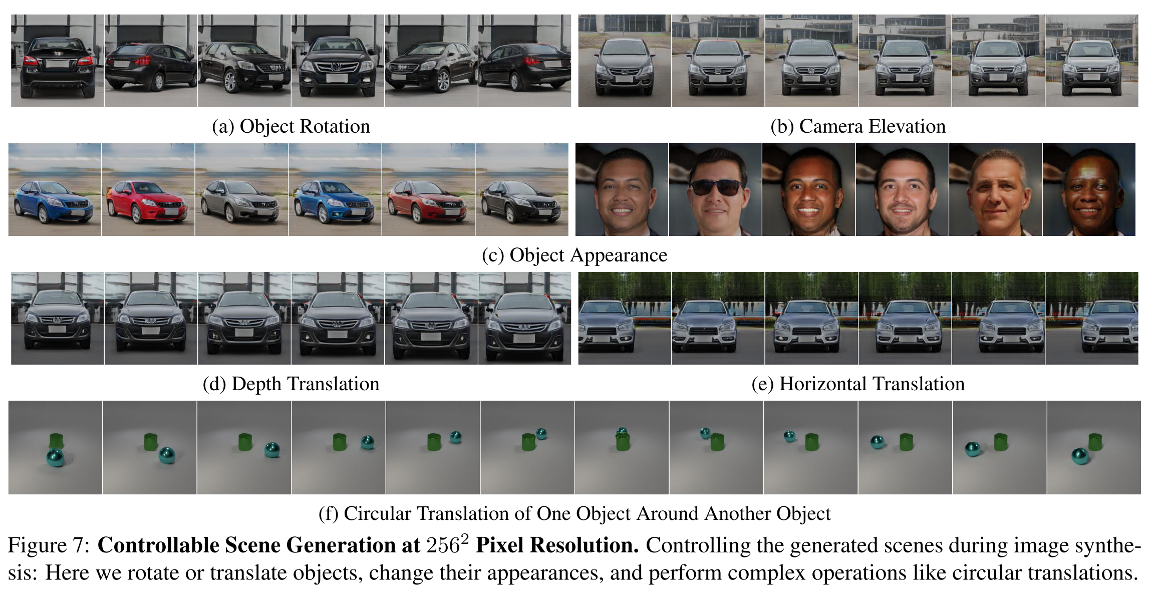
The figure below shows the visual comparions.
Generator
The figure below illustrates the generator. The generator takes four inputs: 3d position x (with frequence encoding), direction d (with frequence encoding), shape embedding \(z_s\) and appearance embedding \(z_a\). The generators are MLP and weights are shared across all subjects. The shape and appearance embedding are learned as part of the algorithm.
We use 8 layers with a hidden dimension of 128 and a density and a feature head of dimensionality 1 and \(M_f = 128\), respectively. For the background feature field \(h^N_{\theta_N}\) , we use half the layers and hidden dimension. We use \(L_x = 2\times 3\times 10\) and \(L_d = 2\times 3\times 4\) for the positional encodings.
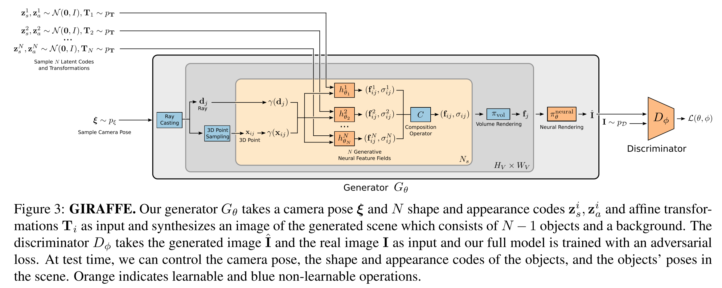
Scene Composition
To composite all the objects to the background, a sum operator is applied:
\[C(x,d)=(\sigma,\frac{1}{\sigma}\sum_i{\sigma_i f_i})\mbox{ where }\sigma=\sum_i{\sigma_i}\]Scene Rendering
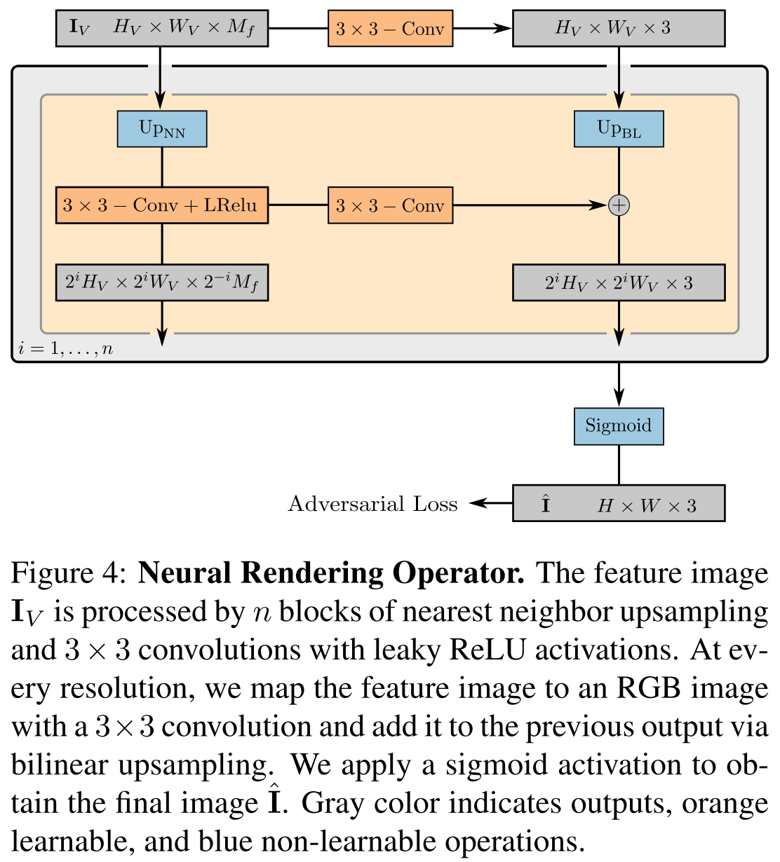
For efficiency, we render feature images at resolution 16x16 which is lower than the output resolution of 64x64 or 256x256 pixels. We then upsample the low-resolution feature maps to higher-resolution RGB images using 2D neural rendering. As evidenced by our experiments, this has two advantages: increased rendering speed and improved image quality.
This render is a 2D convolutional neural network (CNN) with leaky ReLU [56, 89] activation (Fig. 4) and combine nearest neighbor upsampling with 3 × 3 convolutions to in- crease the spatial resolution. We choose small kernel sizes and no intermediate layers to only allow for spatially small refinements to avoid entangling global scene properties during image synthesis while at the same time allowing for in- creased output resolutions. Inspired by [40], we map the feature image to an RGB image at every spatial resolution, and add the previous output to the next via bilinear upsampling. These skip connections ensure a strong gradient flow to the feature fields. We obtain our final image prediction by applying a sigmoid activation to the last RGB layer.
The figure below shows the one layer of this render.
Loss Function
Different from other NeRF which uses L2 or L1 as loss function, this method is a CNN as discriminator.