HeadNeRF A Real-time NeRF-based Parametric Head Model
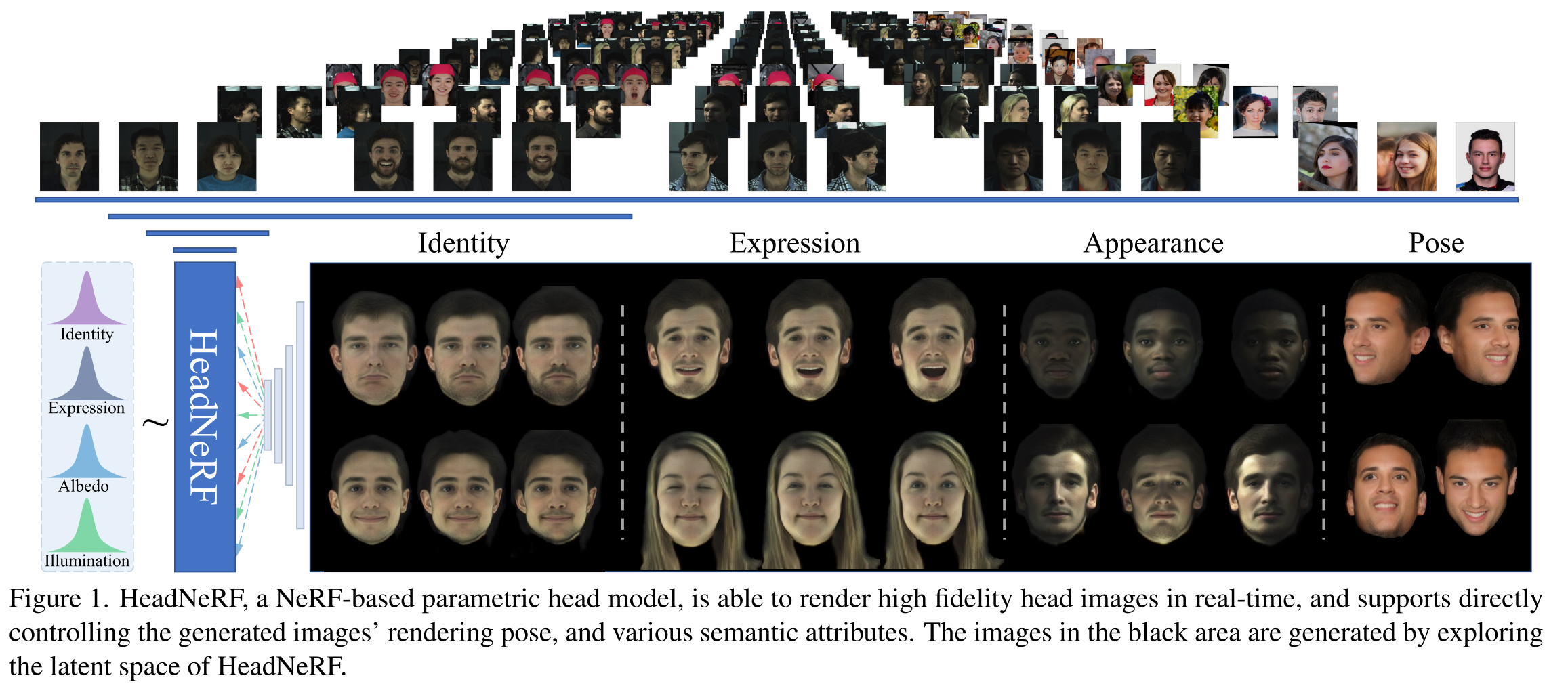
[lighting albedo 3dmm headnerf cnn mlp nerf deep-learning illumination differential-rendering pose expression identity HeadNeRF: A Real-time NeRF-based Parametric Head Model provides a parametric head model which could generates photorealistic face images conditioned on identity, expression, head pose and appearance (lighting). Compared with traditional mesh and texture, it provides higher fidelity, inherently differetiable and doesn’t required a 3D dataset; compared with GAN, it provides rendering at different head pose with accurate 3D information. This is achived with NeRF. In addition, it could render in real time (5ms) with a model GPU.
The major contributions of HeadNeRF are:
- We propose the first NeRF-based parametric human head model, which can directly efficiently control the rendering pose, identity, expression, and appearance.
- We propose an effective training strategy to train the model from general 2D image datasets, and the trained model can generate high fidelity rendered images.
- We design and implement several novel applications with HeadNeRF, and the results verify its effective- ness. We believe that more interesting applications can be explored with our HeadNeRF.
Network Architecture
The network of HeadNeRF could be described as below. Similar to 3DMM, we consider that the underlying geometric shape of the head image is mainly controlled by latent codes related to identity and expression, and the latent codes of albedo and illumination are responsible for the appearance of rendered heads.
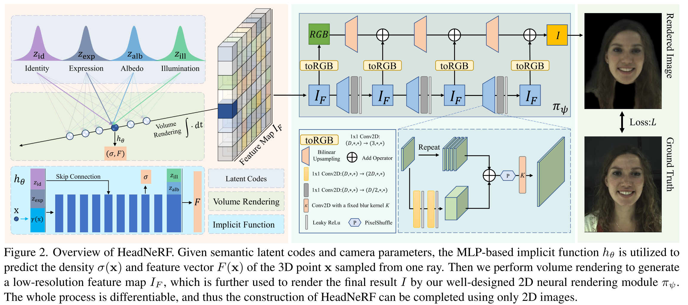
Like previous works [16, 38, 63], instead of directly predicting x’s RGB, we predict a high-dimensional feature vector \(F(x) \in\mathbb{R}^256\) for the 3D sampling point x. Specifically, \(h_\theta\) takes as input the concatenation of \(\gamma(x)\), \(z_{id}\), \(z_{exp}\) and output the density \(\sigma\) of x and an intermediate feature, the latter and \(z_{alb}\), \(z_{ill}\) are used to further predict F(x). Thus, the prediction of the density field is mainly affected by the identity and expres- sion code. The albedo and illumination codes only affect the feature vector prediction.
\[h_\theta:(\gamma(x),z_{id},z_{exp},z_{alb},z_{ill})\to(\sigma,F)\]Then a low-resolution 2D feature map \(I_F\in\mathbb{R}^{256×32×32}\) can be obtained by the following volume rendering strategy:
\[I_F(r)=\int_0^\infty{w(t)F(r(t))}d_t\mbox{ where }w(t)=e^{-\int_0^t{\sigma(r(s))d_s}\sigma(r(t))}\]Finally, we map \(I_F\) to the final predicted image \(I\in\mathbb{R}^{3×256×256}\) with a 2D neural rendering module \(\pi_\psi\), which is mainly composed of 1x1 Conv2D and leaky ReLU [33] activation layer to alleviate possible multi-view inconsistent artifacts [16]. \(\psi\) denotes the learnable parameters. Similar with the strategy used in StyleNeRF [16], the resolution of \(I_F\) is gradually increased through a series of upsampling layers. The upsampling process can be formulated as:
\[\begin{align*} \mbox{Upsample}(X) &= \mbox{Conv2d}(Y,K) \\ Y&=\mbox{Pixelshuffle}(\mbox{repeat}(X,4)+\beta_\zeta(X),2) \end{align*}\]where \(\beta_\zeta : \mathbb{R}^D \to \mathbb{R}^{4D}\) is a learnable 2-layer MLP, ζ denotes the learnable weights, and K is a fixed blur kernel [62]. Like GIRAFFE [38], we map each feature tensor to an RGB image and take the sum of all RGB as the final predicted image. The difference is that we use 1x1 convolution instead of 3x3 convolution to avoid possible multi-view inconsistencies [16].
Latent Codes and Canonical Coordinate
To efficiently train HeadNeRF, we utilize the 3DMM to initialize the latent codes of each image of our training dataset. Although the initial identity code of 3DMM only describes the geometry of the face area (without hair, teeth, etc.), it will be adaptively adjusted through the backpropagation gradient of training.
To this end, for each image, we solve the above- mentioned 3DMM parameter optimization to obtain its corresponding global rigid transformation \(T\in\mathbb{R}^{4×4}\), which transforms the 3DMM geometry from 3DMM canonical coordinate to camera coordinate. We further take this transfor- mation as the camera extrinsic parameter of the image. This strategy actually implicitly aligns the underlying geometry of each image to the center of the 3DMM template mesh.
Dataset
Three datasets has been used to train HeadNeRF:
- FaceSEIP Dataset: 51 subjects x 25 expressions x 13 cameras x 4 lighting conditions;
- FaceScape Dataset: 124 subjects x 20 expressions x 10 cameras;
- FFHQ Dataset: 4133 images.
Loss Function
Three loss functions are used by HeadNeRF. Photometric Loss. For each image, it is required that the rendered result of the head area to be consistent with the corresponding real image, this loss term is formulated as:
\[L_{data}=\lVert M_h\odot (R(z_{id},z_{exp},z_{alb},z_{ill},P)-I_{gt})\rVert^2\]
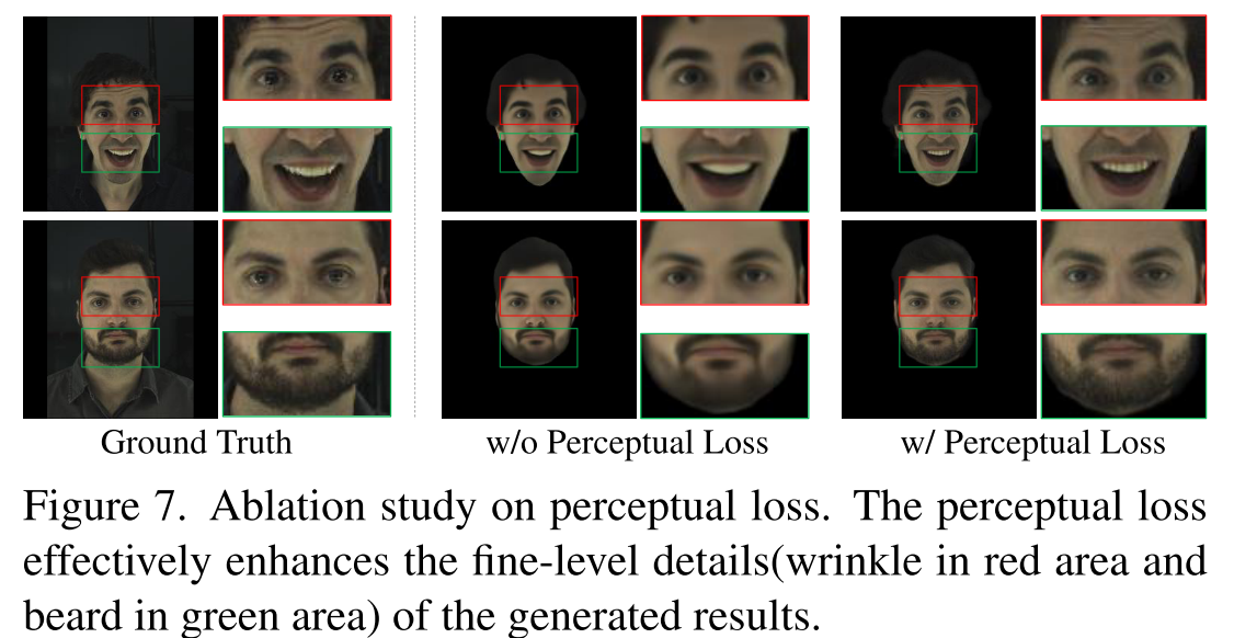
Perceptual Loss. Compared with the vanilla NeRF, Head- NeRF can directly predict the color of all pixels in the rendered image via one inference. Therefore, we adopt the per- ceptual loss [20] in Eq. (6) to further improve the image details of the rendered results.
\[L_{per}=\sum_i{\lVert \phi_i(R(z_{id},z_{exp},z_{alb},z_{ill},P))-\phi_i(I_{gt})\rVert^2}\]where \(\phi_i\) denotes the activation of the i-th layer in VGG16 [46] network. Figure 7 evaluates the impact of this function.
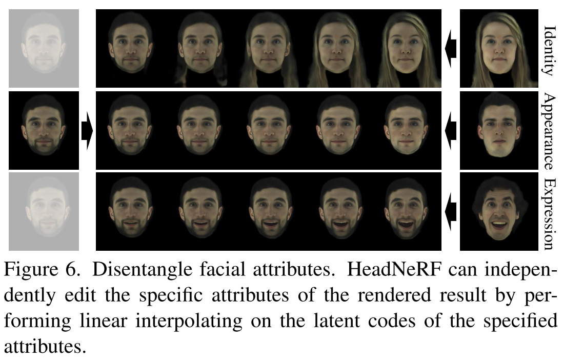
Disentangled Loss. In order to achieve semantically dis- entangled control to the rendered results, we let all images of one subject share the same identity latent code, and the images of the same expression with different lighting conditions and different captured cameras from the same subject share the same expression latent code. To achive this, HeadNeRF requires the latent code as similar as the 3DMM estimation as possible. The impact is shown in Figure 6.
\[L_{dis}=w_{id}\lVert z_{id}-z_{id}^0\rVert^2+w_{exp}\lVert z_{exp}-z_{exp}^0\rVert^2+w_{alb}\lVert z_{alb}-z_{alb}^0\rVert^2+w_{ill}\lVert z_{ill}-z_{ill}^0\rVert^2\]