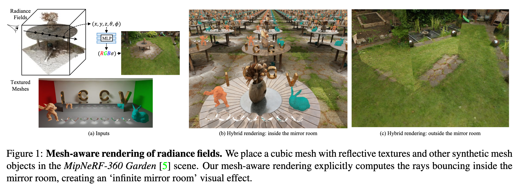
Dynamic Mesh-Aware Radiance Fields
[signed-distance-function iron neuphysics light 3d nerf-studio nerf hdr deep-learning mesh nvdiffrec ray-trace brdf ray-march This is my reading note on Dynamic Mesh-Aware Radiance Fields. This paper proposes a method of rendering NERF with mesh simultaneously. To do that, it modifies the ray trace. To handle occlusion and shadow, SDF is used to represent the surface of NERF and light source is estimated from NERF.
Introduction
Embedding polygonal mesh assets within photorealistic Neural Radience Fields (NeRF) volumes, such that they can be rendered and their dynamics simulated in a physically consistent manner with the NeRF, is under-explored from the system perspective of integrating NeRF into the traditional graphics pipeline. This paper designs a two-way coupling between mesh and NeRF during rendering and simulation. We first review the light transport equations for both mesh and NeRF, then distill them into an efficient algorithm for updating radiance and throughput along a cast ray with an arbitrary number of bounces. To resolve the discrepancy between the linear color space that the path tracer assumes and the sRGB color space that standard NeRF uses, we train NeRF with High Dynamic Range (HDR) images. We also present a strategy to estimate light sources and cast shadows on the NeRF. Finally, we consider how the hybrid surface-volumetric formulation can be efficiently integrated with a high-performance physics simulator that supports cloth, rigid and soft bodies. The full rendering and simulation system can be run on a GPU at interactive rates (p. 1)
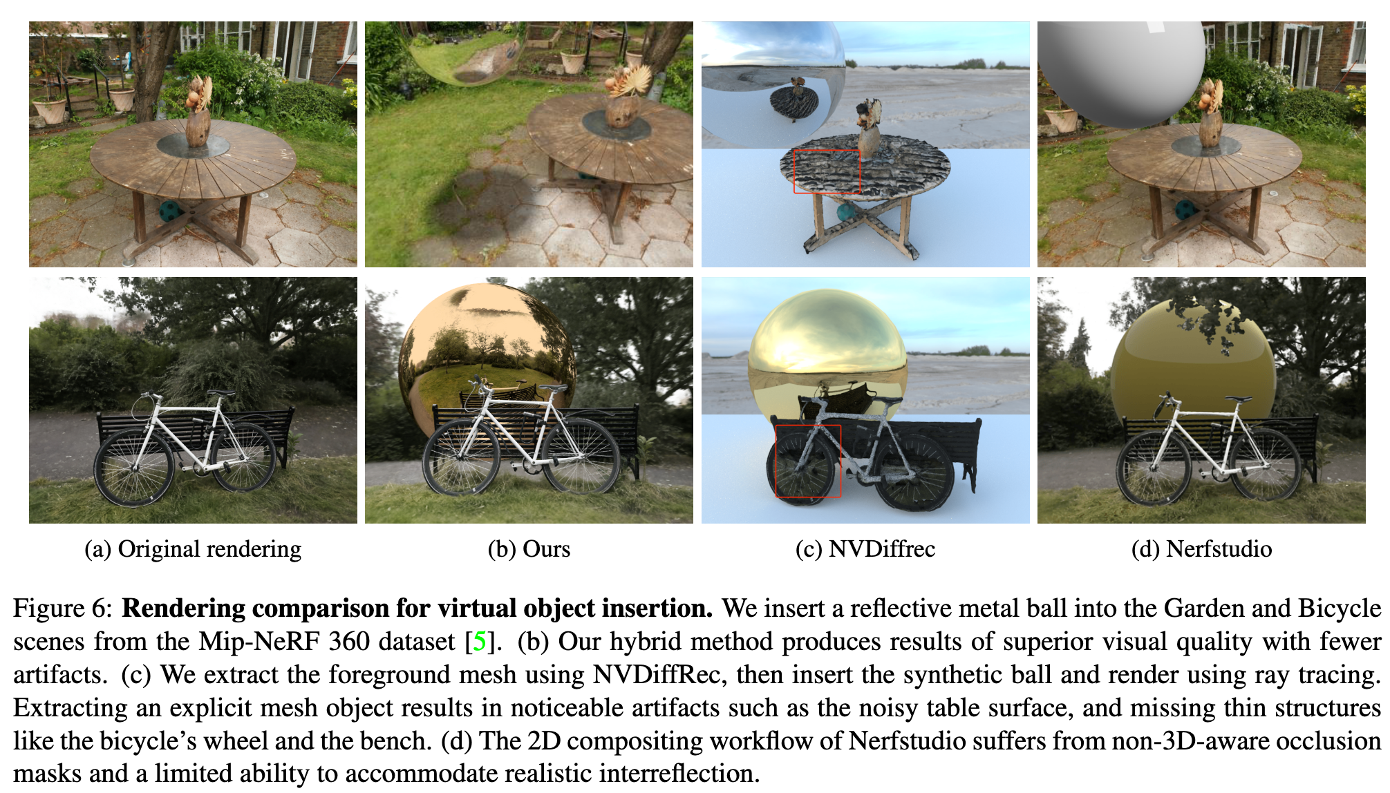
However, integrating NN-based NeRF into this pipeline while maintaining realistic lighting effects such as shadows, reflections, refractions, and more, remains a relatively unexplored area. In terms of simulation, while the geometry of NeRF is implicit in its density field, it lacks a well-defined surface representation, making it difficult to detect and resolve collisions. Recent works have delved into enhancing the integration between NeRF and meshes, aiming to combine the photorealistic capabilities of NeRF with the versatility of meshes for rendering and simulation. Neural implicit surfaces [87, 80, 59, 19] are represented as learned Signed Distance Fields (SDF) within the NeRF framework. Meanwhile, methods like IRON [94] and NVDiffRec [52] extract explicit, textured meshes that are directly compatible with path tracing, offering practical benefits at the expense of a lossy discretization. Nerfstudio [72] renders NeRF and meshes separately, then composites the render passes with an occlusion mask. Unfortunately, this decoupled rendering approach offers no way to exploit the lighting and appearance information encoded in the NeRF volume to affect the rendered mesh appearance (p. 2)
By unifying NeRF volume rendering and path tracing within the linear RGB space, we discover their Light Transport Equations exhibit similarities in terms of variables, forms, and principles. Leveraging their shared light transport behavior, we devise update rules for radiance and throughput variables, enabling seamless integration between NeRF and meshes. To incorporate shadows onto the NeRF, we employ differentiable surface rendering techniques [28] to estimate light sources and introduce secondary shadow rays during the ray marching process to determine visibility. Consequently, the NeRF rendering equation is modified to include a pointwise shadow mask. (p. 2)
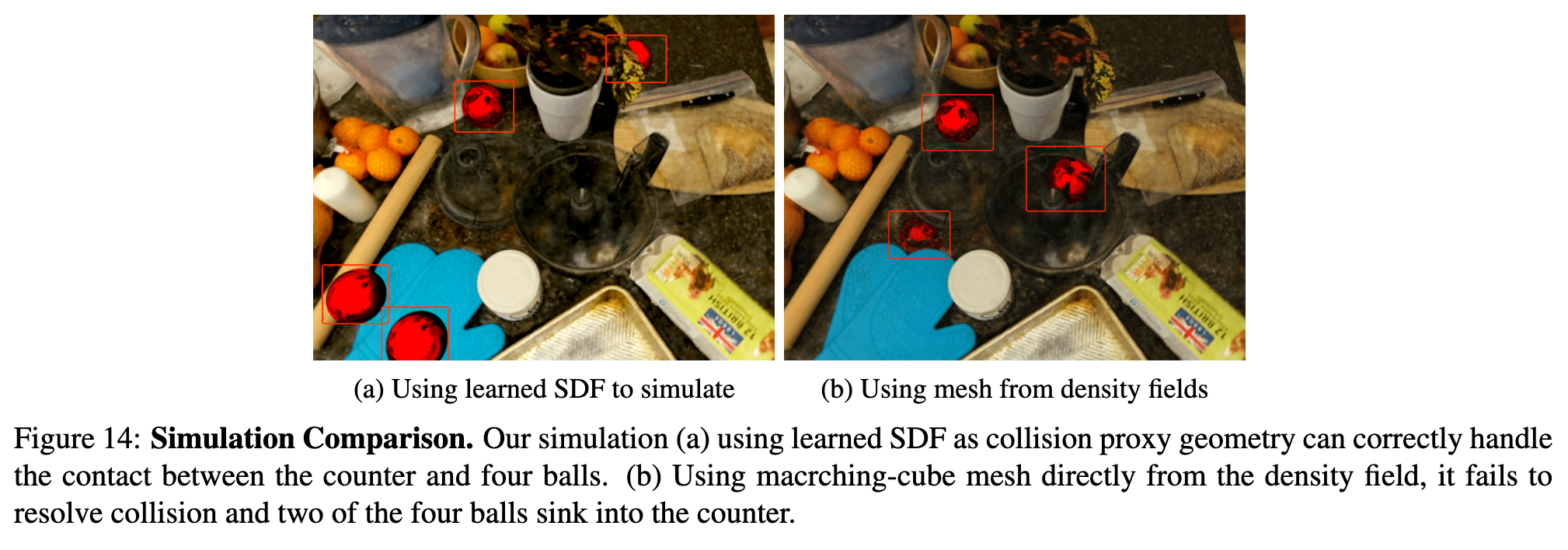
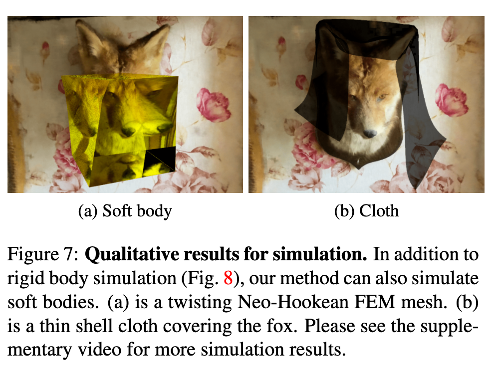
For simulation, we adopt SDFs to represent geometry of neural fields, which is advantageous for physical contact handling and collision resolution. We then use positionbased dynamics [42] for time integration. (p. 2)
Contributions:
- A two-way coupling between NeRF and surface representations for rendering and simulation.
- Integration with HDR data which can unify the color space of the path tracer and NeRF, with a strategy to estimate light sources and cast shadows on NeRF.
- An efficient rendering procedure that alternates ray marching and path tracing steps by blending the Light Transport Equations for both NeRF and meshes.
- An interactive, easy-to-use implementation with a high-level Python interface that connects the low-level rendering and simulation GPU kernels. (p. 2)
Related Work
Neural Fields and Surface Representations
- In rendering, [94] and [52] propose to use surface-based differentiable rendering to reconstruct textured meshes [23] from neural fields. Their reconstructed meshes can be imported to a surface rendering pipeline like Blender [15], but the original NeRF representation cannot be directly rendered with meshes.
- For simulation, NeRFEditting [92] proposes to use explicit mesh extracted by [80] to control the deformation of Neural Fields.
- Qiao et al. [65] further add full dynamics over the extracted tetrahedra mesh.
- Chu et al. [13] integrates the dynamics of smoke with neural fields.
- [14] also connects differentiable simulation to NeRF, where the density field and its gradient are used to compute the contact. These methods aim to construct an end-to-end differentiable simulation and rendering pipeline, yet they have yet to couple the rendering (p. 3)
Scene Editing and Synthesis:
- For neural field representations, ray bending [75, 64, 34] is widely used to modify an optimized NeRF. It is possible to delete, add, duplicate, or actuate [10, 62, 82, 37] an area by bending the path of the rendering ray.
- [22] propose to train a NeRF for each object and compose them into a scene.
- ClimateNeRF [35] can change weather effects by modifying the density and radiance functions during ray marching. These methods study editing of isolated NeRF models.
- There are also inverse rendering works that decompose [86, 6] the information baked into NeRF, which can then be used to edit lighting and materials [32]. Such decomposition is useful, but assumes information like a priori knowledge of light sources, or synthetic scenes. They do not address inserting mesh into NeRF scenes.
- Besides NeRF, [30] inserts a virtual object into existing images by estimating the geometry and light source in the existing image. [11] insert vehicles in street scenes by warping textured cars using predicted 3D poses. (p. 3)
There are two recent works [14, 65] that can simulate in neural fields.
- [14] establish a collision model based on the density field. In our simulation, we found that the density fields are usually noisy and inadequate to model a surface well for accurate contact processing.
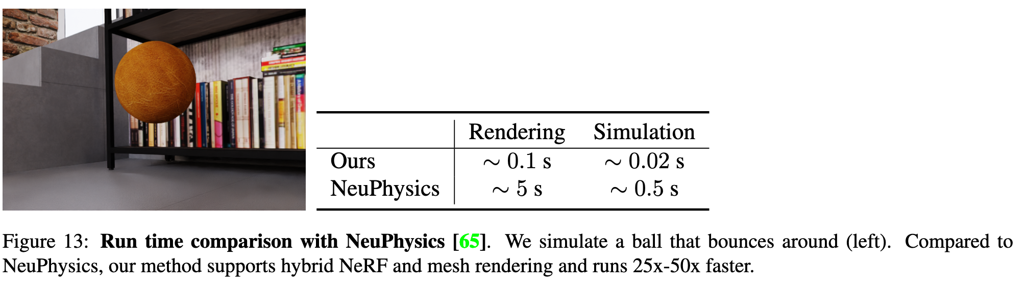
- NeuPhysics[65] aims at differentiable simulation and rendering, and it extracts hexahedra mesh from learned SDF [80] and simulates the mesh using [18]. NeuPhysics can only simulate existing NeRF objects instead of synthetic objects. Table 13 shows that our method runs at least an order of magnitude faster when simulating a bouncing ball. (p. 13)
Rendering
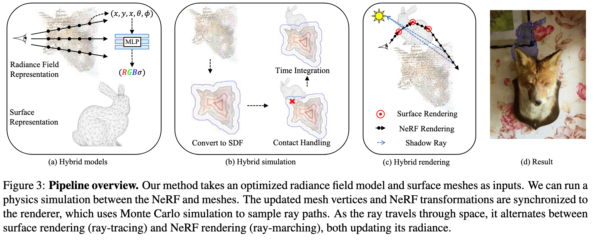
One possible approach to bridge these disparate representations is to render the meshes and NeRF volume in separate passes, and composite the results together in 2D image space. However, compositing in image space is susceptible to incorrect occlusion masks and inaccurate lighting. A more physically principled approach to this problem is identifying and exploiting the similarities in their respective light transport equations, which directly allows the radiance field and mesh to be incorporated in 3D space. (p. 3)
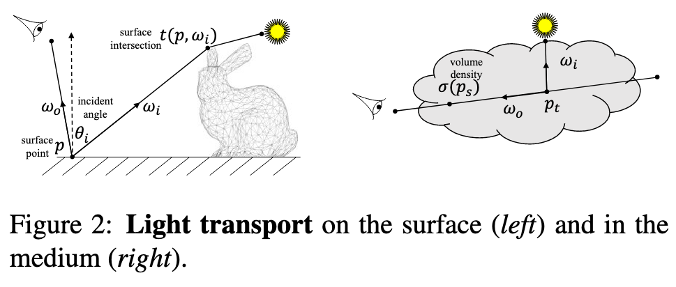
Surface Rendering Equation
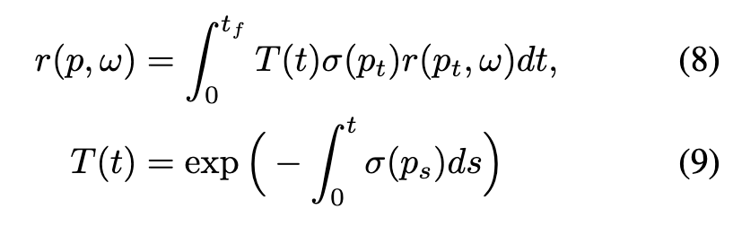
The Light Transport Equation (LTE) for surface rendering is: (p. 3)
where p is a surface point; ωi, ωo are the directions of incident (incoming) and exitant (outgoing) radiance; S2 is the unit sphere sampling space for directions; L, Le, Li, Lr are the exitant, emitted, incident, and reflected radiance, respectively; θi is the angle of incidence of illumination; fs(p, ωo, ωi) is the bidirectional scattering distribution function (BSDF); and t(p, ω) is the ray-casting function that computes the first surface intersected by the ray cast from p in the direction ω. (p. 3)
If a scene is represented solely by surfaces, the LTE in Equation 1 can be solved by Monte Carlo path tracing: for each pixel, a ray is randomly cast from the camera, its path constructed incrementally each time it hits, and bounces off of a surface. (p. 4)
Volumetric Rendering Equation
The light transport equation for the volumetric medium is: (p. 4)
where Ls is the (weighted) scattered radiance, σt and σs are the attenuations and scattering coefficients, fp is the phase function of the volume, and ps is on the ray ps = p + s · ωo (similar to pt). All other terms share the same definition as in surface rendering. (p. 4)
The integral in the volumetric LTE could again be solved using Monte Carlo methods. However, stochastic simulation of volumetric data is more challenging and expensive than surface data. A photon may change direction in a continuous medium, unlike the discrete bounces that occur only at surfaces. Therefore, rather than simulating the path of photons using Monte Carlo sampling, methods like NeRF [46] instead bake the attenuation coefficient σ(p) = σt(p) and view-dependent radiance r(p, ω) onto each spatial point, and so there is no scattering. This circumvents solving Equation 7, thereby avoiding considering light transport, light sources, and material properties. Volume rendering under the NeRF formulation becomes: (p. 4)
Color Space
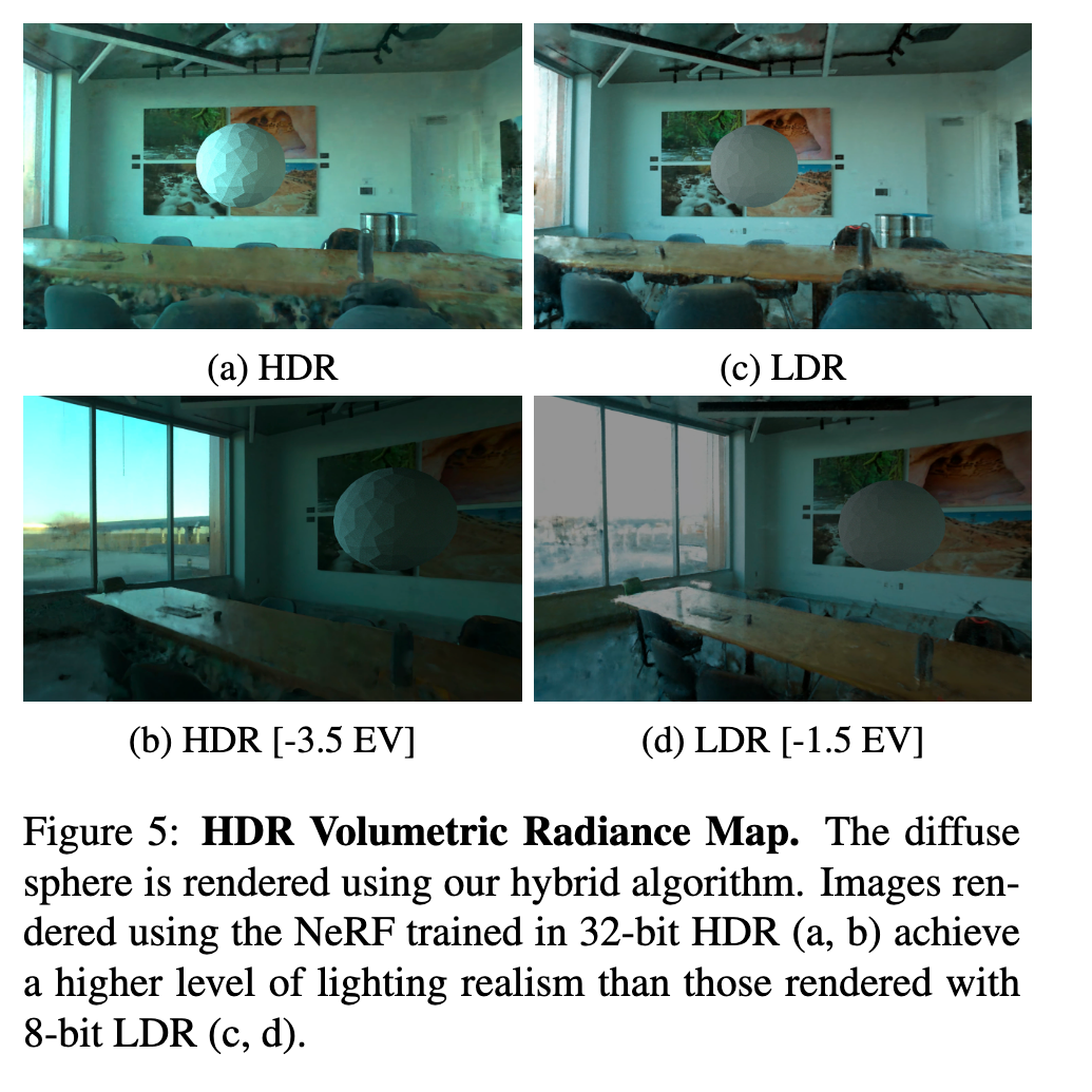
To reconcile this difference, we train an HDR variant of NeRF, supervised with 32-bit HDR images directly rather than the standard 8-bit NeRF. The resulting HDR NeRF produces a 3channel radiance in 32-bit linear color space at each sampled point. (p. 5)
To create a single one of these HDR images, we shoot a bracketed series of LDR exposures that consists of several images (7 in our experiments) captured from a fixed camera pose. We use a single Canon 5D MKIII with a 28mm lens, and set the camera to record images in 8-bit JPEG format. (p. 14)
Estimating light sources
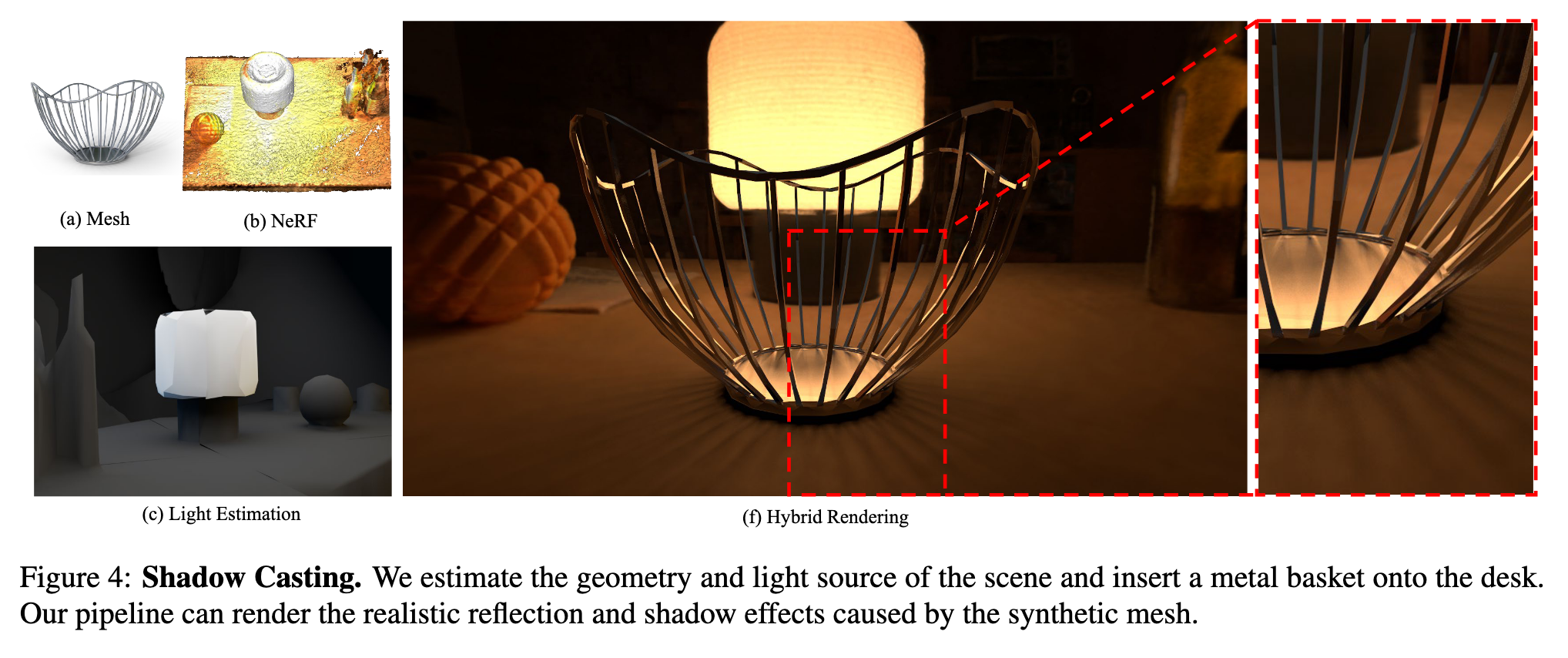
Note that NeRF’s volume rendering formulation bakes appearance into each point in the volume rather than simulating physically based light transport. To recover an explicit representation of light sources, we first reconstruct the scene’s geometry as a neural SDF using MonoSDF [91], from which we extract an explicit mesh. Then, we employ a differentiable path tracer, Mitsuba3 [28, 29], to estimate a UV Emission Texture for the mesh. (p. 5)
Once the light source estimation has converged, we prune faces whose emission falls below a threshold from the explicit mesh, which is necessary for efficiency (p. 5)
Shadow rays
We query additional rays during ray marching to cast shadows on NeRF. For each sampled point pt in NeRF, we shoot a secondary ray from pt to the light source (see the following subsection for details on estimating lighting sources). If an inserted mesh blocks this ray, then this pt has a shadow mask m(pt) = 1 − rsrc, where rsrc is the intensity of the light source. Non-blocked pixels have mshadow = 1 (p. 5)
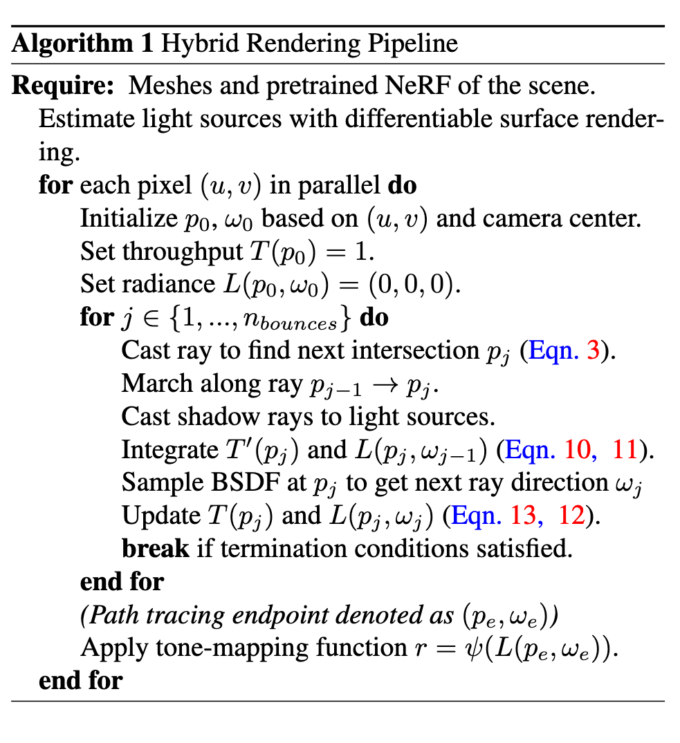
Hybrid Rendering Algorithm
The differences are: (1) Surface rendering updates those values on discrete boundaries while NeRF accumulates them in the continuous space; (2) T(p) and r(p, ω) are governed by the BSDF parameters in surface rendering, while by neural fields in NeRF. Therefore, we can alternate between the surface and NeRF rendering rules as they travel in space (p. 5)
Simulation
Neural fields and meshes can be connected in the simulation pipeline by Signed Distance Fields (SDF) or reconstructed surface mesh (p. 6)
We employ extended position-based dynamics (XPBD) [43, 48] to simulate the objects during runtime. We choose this dynamics model because it is fast and can support various physical properties. Collision detection is performed by querying the SDF of all vertices. (p. 6)
We can get the homogenous transformation t ∈ R4×4 of the NeRF from simulation in each time step, which is used to inverse transform the homogenous coordinates t−1 ·p [64] when querying the color/density and sampling rays in the Instant-NGP hash grid (p. 6)
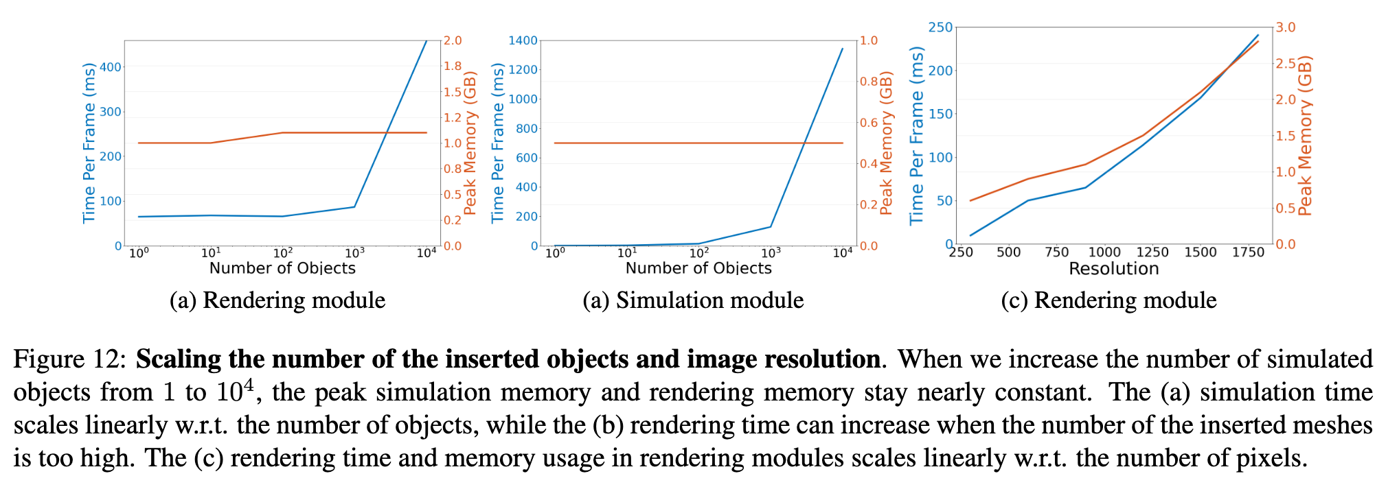
Our method can achieve a runtime of 1 to 40 frames per second, contingent upon the resolution, scene complexity, and dynamics (p. 7)
Experiment
Moreover, the simulation module is independent of the resolution, and the rendering time scales linearly w.r.t. the number of pixels (see left). This pipeline can run in real time (20 FPS) at 600 × 300 resolution. (p. 13)