MVSNeRF Fast Generalizable Radiance Field Reconstruction from Multi-View Stereo
[nerf mvs-nerf deep-learning mvsnet multi-view-stereo This is my reading note for MVSNeRF: Fast Generalizable Radiance Field Reconstruction from Multi-View Stereo. It first build a cost volume at the reference view (we refer to the view i = 1 as the reference view) by warping 2D neural features onto multiple sweeping planes (Sec. 3.1). It then leverage a 3D CNN to reconstruct the neural encoding volume, and use an MLP to regress volume rendering properties, expressing a radiance field (Sec. 3.2). It leverage differentiable ray marching to regress images at novel viewpoints using the radiance field modeled by the network; this enables end-to-end training of our entire framework with a rendering loss (Sec. 3.3)
Introduction
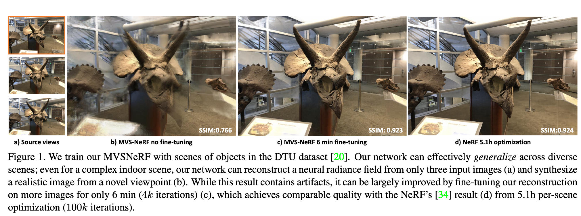
Unlike prior works on neural radiance fields that consider per-scene optimization on densely captured images, we propose a generic deep neural network that can reconstruct radiance fields from only three nearby input views via fast network inference. Our approach leverages plane-swept cost volumes (widely used in multi-view stereo) for geometry-aware scene reasoning, and combines this with physically based volume rendering for neural radiance field reconstruction (p. 1)
We propose MVSNeRF, a novel approach that generalizes well across scenes for the task of reconstructing a radiance field from only several (as few as three) unstructured multi-view input images (p. 2)
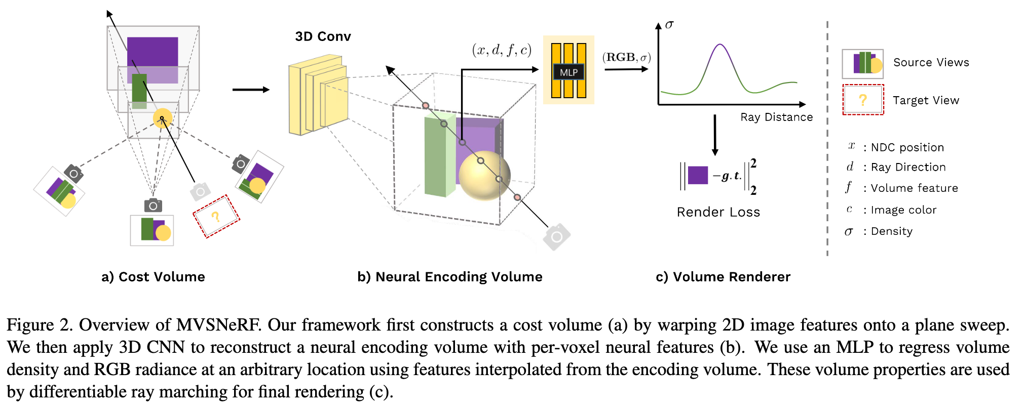
We take advantage of the recent success on deep multi- view stereo (MVS) [50, 18, 10]. This line of work can train generalizable neural networks for the task of 3D reconstruction by applying 3D convolutions on cost volumes. Similar to [50], we build a cost volume at the input reference view by warping 2D image features (inferred by a 2D CNN) from nearby input views onto sweeping planes in the reference view’s frustrum. Unlike MVS methods [50, 10] that merely conduct depth inference on such a cost volume, our network reasons about both scene geometry and appearance, and outputs a neural radiance field (see Fig. 2), enabling view synthesis. Specifically, leveraging 3D CNN, we reconstruct (from the cost volume) a neural scene encoding volume that consists of per-voxel neural features that encode information about the local scene geometry and appearance. Then, we make use of a multi-layer perceptron (MLP) to decode the volume density and radiance at arbitrary continuous locations using tri- linearly interpolated neural features inside the encoding volume. In essence, the encoding volume is a localized neural representation of the radiance field; once estimated, this volume can be used directly (dropping the 3D CNN) for final rendering by differentiable ray marching (as in [34]). (p. 2)
Proposed Method
In general, our entire network can be seen as a function of a radiance field, expressed by:
 where x represents a 3D location, d is a viewing direction, σ is the volume density at x, and r is the output radiance (RGB color) at x depending on the viewing direction d.The output volume properties from our network can bedirectly used to synthesize a novel image It at a novel target viewpoint Φt via differentiable ray marching. (p. 3)
The overview of our MVSNeRF is shown in Fig. 2. We first build a cost volume at the reference view (we refer to the view i = 1 as the reference view) by warping 2D neural features onto multiple sweeping planes (Sec. 3.1). We then leverage a 3D CNN to reconstruct the neural encoding volume, and use an MLP to regress volume rendering properties, expressing a radiance field (Sec. 3.2). We leverage differentiable ray marching to regress images at novel viewpoints using the radiance field modeled by our network; this enables end-to-end training of our entire framework with a rendering loss (Sec. 3.3) (p. 3)
Cost volume construction
The cost volume P is constructed from the warped feature maps on the D sweeping planes. We leverage the variance-based metric to compute the cost, (p. 4)

where Var computes the variance across M views. (p. 4)
Radiance field reconstruction
We utilize a 3D CNN B to reconstruct a neural encoding volume S from the cost volume P of raw 2D image feature costs; S consists of per-voxel features that encode local scene geometry and appearance. An MLP decoder A is used to regress volume rendering properties from this encoding volume. (p. 4)
The 3D CNN B is a 3D UNet with downsampling and upsampling convolutional layers and skip connections, which can effectively infer and propagate scene appearance information, leading to a meaningful scene encoding volume S. Note that, this encoding volume is predicted in a unsupervised way and inferred in the end-to-end training with volume rendering (p. 4)
The scene encoding volume is of relative low resolution because of the downsampling of 2D feature extraction; it is challenging to regress high-frequency appearance from this information alone. We thus also incorporate the original image pixel data for the following volume regression stage (p. 4)
we also consider pixel colors c = [I(ui, vi)] from the original images Ii as additional input; here (ui, vi) is the pixel location when projecting the 3D point x onto view i, and c concatenates the colors I(ui, vi) from all views as a 3M-channel vector (p. 4)
Volume rendering and end-to-end training
This ray marching rendering is fully differentiable; it thus allows our framework to regress final pixel colors at novel viewpoints using the three input views from end to end. We supervise our entire framework with the groundtruth pixel colors, using an L2 rendering loss: (p. 5)
Optimizing the neural encoding volume
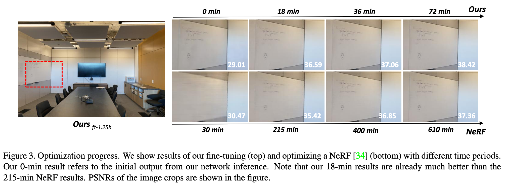
In contrast, we propose to fine-tune our neural encoding volume – that can be instantly reconstructed by our network from only few images – to achieve fast per-scene optimization when dense images are captured. (p. 5)
We instead achieve an independent neural reconstruction by appending the per-view colors of voxel centers as additional channels to the encoding volume; (p. 5)
Note that, we optimize only the encoding volume and the MLP, instead of our entire network (p. 5)
Experiment
