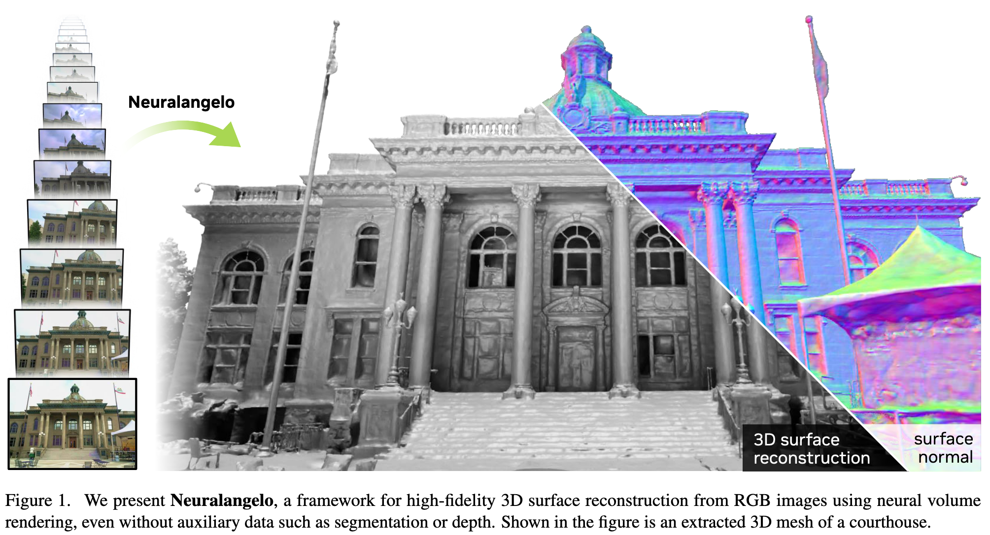
Neuralangelo High-Fidelity Neural Surface Reconstruction
[nerf deep-learning instant-ngp 3d This is my reading note on Neuralangelo: High-Fidelity Neural Surface Reconstruction. This paper proposes a method to reconstruct 3D surface at very high details. The proposed method is based on two improvements: 1) use numerical gradient instead of analytical one to remove non locality 2) use multi resolution instant NGP improve details from coarse to fine.
Introduction
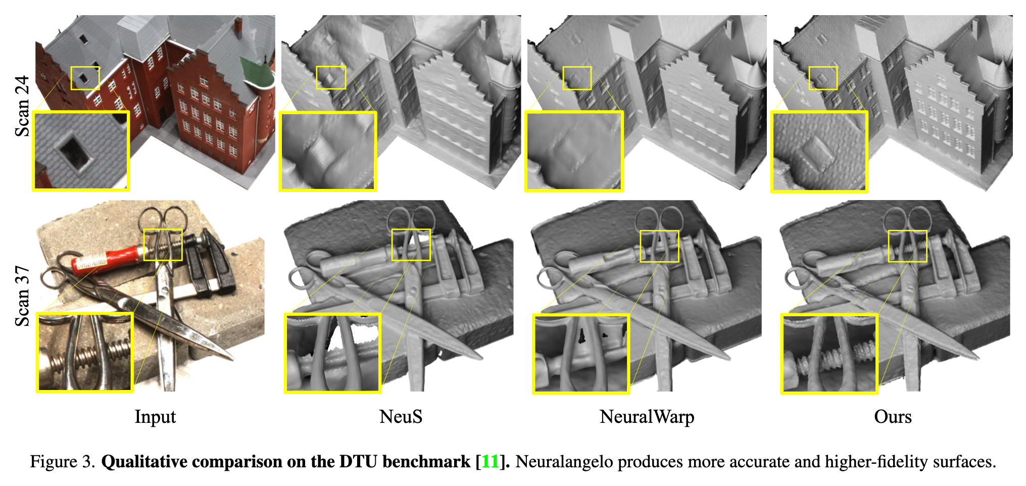
However, current methods struggle to recover detailed structures of real-world scenes. To address the issue, we present Neuralangelo, which combines the representation power of multi-resolution 3D hash grids with neural surface rendering. Two key ingredients enable our approach: (1) numerical gradients for computing higher-order derivatives as a smoothing operation and (2) coarse-to-fine optimization on the hash grids controlling different levels of details. (p. 1)
Neural surface reconstruction. For scene representations with better-defined 3D surfaces, implicit functions such as occupancy grids [27, 28] or SDFs [48] are preferred over simple volume density fields. (p. 2)
Preliminaries
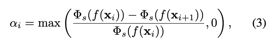
Wang et al. [41] proposed to convert volume density predictions in NeRF to SDF representations with a logistic function to allow optimization with neural volume rendering. Given a 3D point xi and SDF value f(xi), the corresponding opacity value αi used in Eq. 1 is computed as (p. 3)
The hash encoding uses multi-resolution grids, with each grid cell corner mapped to a hash entry. Each hash entry stores the encoding feature. Let {V1, …, VL} be the set of different spatial grid resolutions. Given an input position xi, we map it to the corresponding position at each grid resolution Vl as xi,l = xi · Vl. The feature vector $\gmma_l(x_i,l) \in R^c$ given resolution Vl is obtained via trilinear interpolation of hash entries at the grid cell corners. The encoding features across all spatial resolutions are concatenated together, forming a $\gamma(x_i) \in R^{cL}$ feature vector. The encoded features are then passed to a shallow MLP. (p. 3)
Numerical Gradient Computation
We show in this section that the analytical gradient w.r.t. position of hash encoding suffers from localities. Therefore, optimization updates only propagate to local hash grids, lacking non-local smoothness. We propose a simple fix to such a locality problem by using numerical gradients. An overview is shown in Fig. 2. (p. 3)
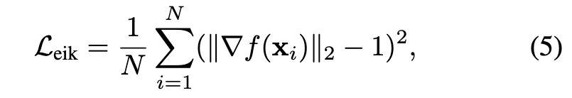
A special property of SDF is its differentiability with a gradient of the unit norm. The gradient of SDF satisfies the eikonal equation ∥∇f(x)∥2 = 1 (almost everywhere). To enforce the optimized neural representation to be a valid SDF, the eikonal loss [8] is typically imposed on the SDF predictions: (p. 3)
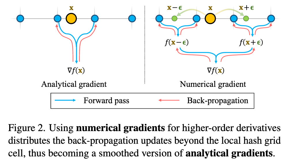
If the step size of the numerical gradient is smaller than the grid size of hash encoding, the numerical gradient would be equivalent to the analytical gradient; otherwise, hash entries of multiple grid cells would participate in the surface normal computation (p. 4)
Intuitively, numerical gradients with carefully chosen step sizes can be interpreted as a smoothing operation on the analytical gradient expression. An alternative of normal supervision is a teacher-student curriculum [40, 54], where the predicted noisy normals are driven towards MLP outputs to exploit the smoothness of MLPs. However, analytical gradients from such teacher-student losses still only back-propagate to local grid cells for hash encoding. In contrast, numerical gradients solve the locality issue without the need of additional networks. (p. 4)
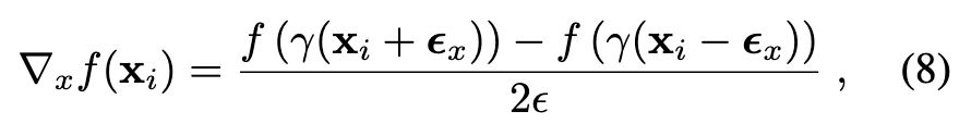
To compute the surface normals using the numerical gradient, additional SDF samples are needed. Given a sampled point xi = (xi, yi, zi), we additionally sample two points along each axis of the canonical coordinate around xi within a vicinity of a step size of ϵ. For example, the x-component of the surface normal can be found as (p. 4)
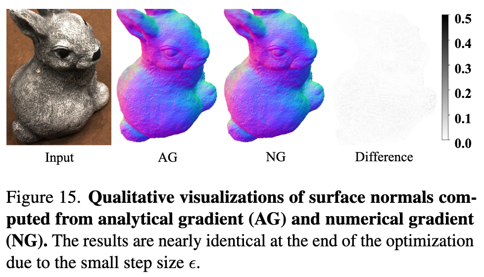
At the end of the optimization, the step size ϵ has decreased sufficiently small to the grid size of the finest hash resolution. Using numerical gradients is nearly identical to using analytical gradients. Fig. 15 shows that the surface normals computed from both numerical and analytical gradients are indeed qualitatively similar, with negligible errors scattered across the object. (p. 14)
Progressive Levels of Details
Imposing L_eik with a larger ϵ for numerical surface normal computation ensures the surface normal is consistent at a larger scale, thus producing consistent and continuous surfaces. On the other hand, imposing L_eik with a smaller ϵ affects a smaller region and avoids smoothing details. In practice, we initialize the step size ϵ to the coarsest hash grid size and exponentially decrease it matching different hash grid sizes throughout the optimization process. (p. 4)
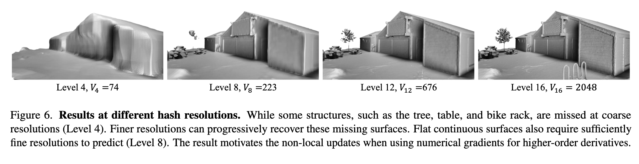
Therefore, we only enable an initial set of coarse hash grids and progressively activate finer hash grids throughout optimization when ϵ decreases to their spatial size. The relearning process can thus be avoided to better capture the details. In (p. 5)
Optimization
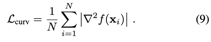
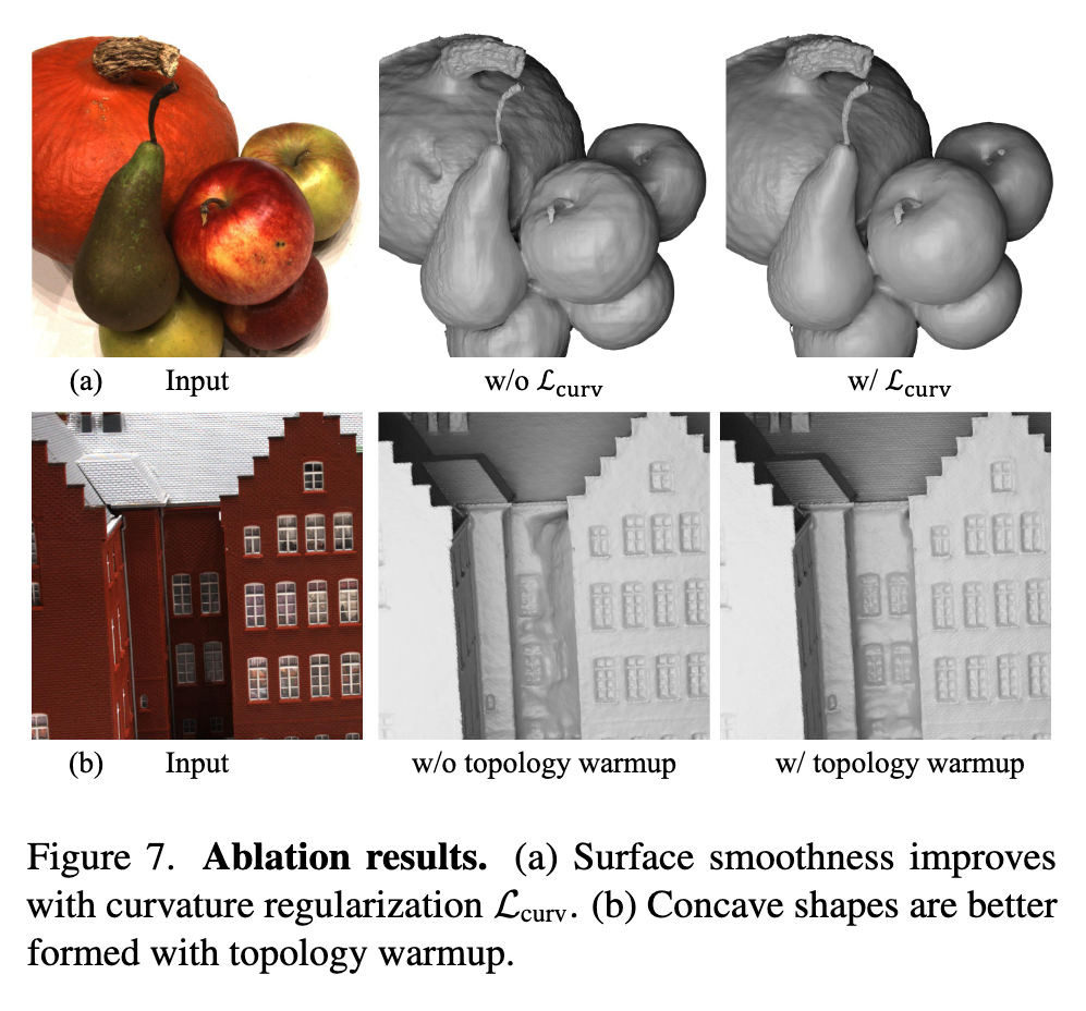
To further encourage the smoothness of the reconstructed surfaces, we impose a prior by regularizing the mean curvature of SDF. The mean curvature is computed from discrete Laplacian similar to the surface normal computation (p. 5)
Implementation details. Our hash encoding resolution spans 25 to 211 with 16 levels. Each hash entry has a channel size of 8. The maximum number of hash entries of each resolution is 222. We activate 4 and 8 hash resolutions at the beginning of optimization for DTU dataset and Tanks and Temples respectively, due to differences in scene scales. We enable a new hash resolution every 5000 iterations when the step size ϵ equals its grid cell size (p. 5)
Experiment
Ablation
Topology warmup.
We follow prior work and initialize the SDF approximately as a sphere [48]. With an initial spherical shape, using Lcurv also makes concave shapes difficult to form because Lcurv preserves topology by preventing singularities in curvature. Thus, instead of applying Lcurv from the beginning of the optimization process, we use a short warmup period that linearly increases the curvature loss strength. (p. 8)
Color network
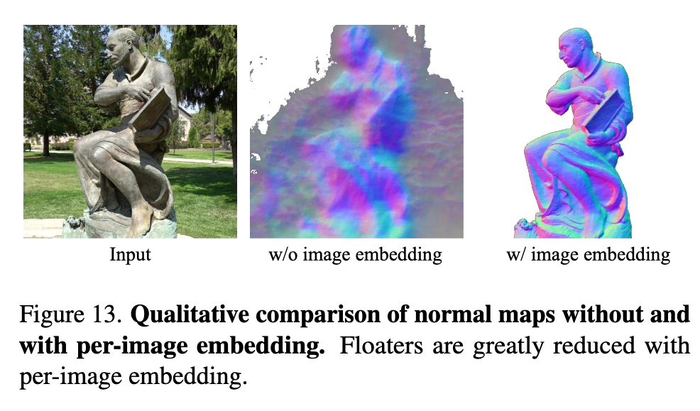
For the Tanks and Temples dataset, we add per-image latent embedding to the color network following NeRF-W [24] to model the exposure variation across frames. (p. 14)
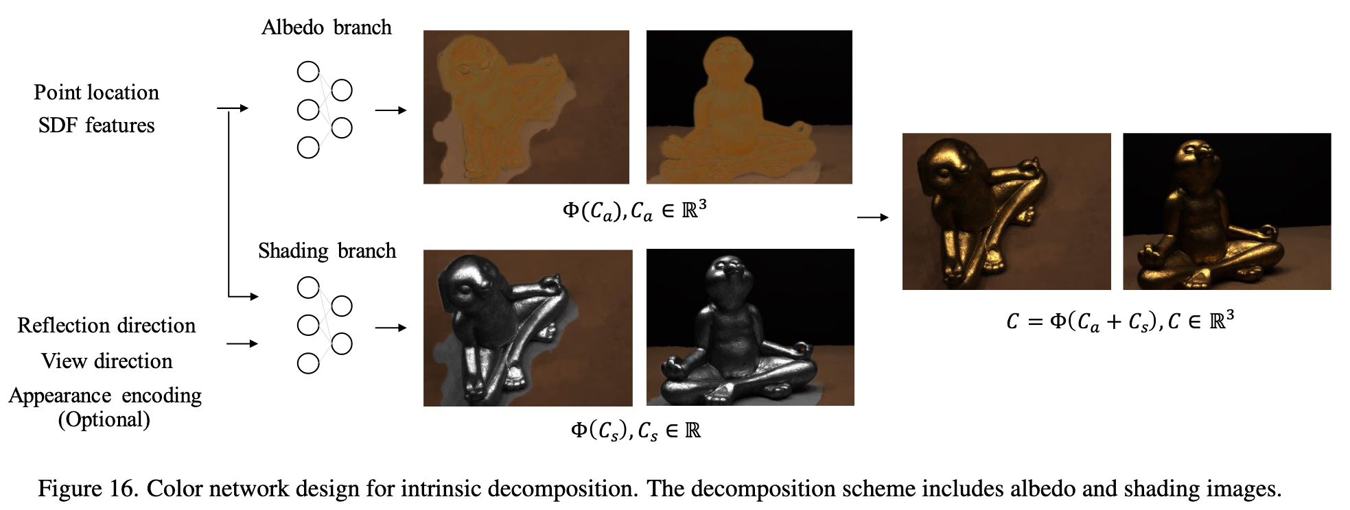
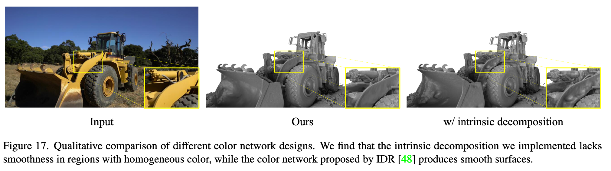
However, we do not observe improvements in surface qualities using such a decomposition design. The intrinsic decomposed color network contains two branches – albedo and shading branches. The final rendered image C ∈ R3 is the sum of the albedo image Ca and shading image Cs: (p. 14)
The albedo branch predicts RGB values Ca ∈ R3 that are view-invariant. It receives point locations and features from the SDF MLP as input. On the other hand, the shading branch predicts gray values Cs ∈ R that is view dependent to capture reflection, varying shadow, and exposure changes. (p. 14)
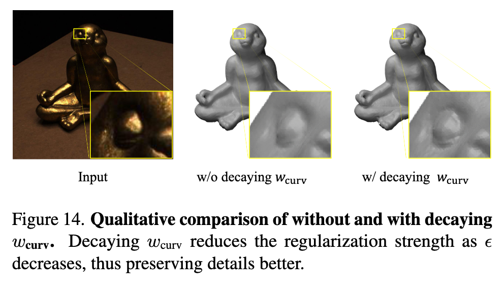
Curvature regularization strength
As the step size ϵ decreases and finer hash grids are activated, finer details may be smoothed if the curvature regularization is too strong. To avoid loss of details, we scale down the curvature regularization strength by the spacing factor between hash resolutions each time the step size ϵ decreases. (p. 14)