Get Option Data from Yahoo with Pandas

[ option  pandas  finance  ]

This notebook shows how to read the option chain data from Yahoo finance with Pandas. Especially we will use pandas.read_html.

Import some Libraries

First, let us import some library

import pandas as pd
from matplotlib import pyplot as plt
import matplotlib
from datetime import datetime
import numpy as np


%matplotlib inline
plt.rcParams['figure.figsize'] = [20, 10]

Get the Right Url

If we want to get Tesla option data for Mar 5th 2021 from Yahoo finance, we need to visit this url https://finance.yahoo.com/quote/TSLA/options?date=1614902400. TSLA is the ticket name for Tesla and 1614902400 is the unix epoch seconds for Mar 5th 2021. So we have this function

def get_url(tick: str, year: int, month: int, day: int) -> str:
  """Get url for the Yahoo option chain table"""
  date = int(datetime(year, month, day).timestamp())
  tick = tick.upper()
  return f"https://finance.yahoo.com/quote/{tick}/options?date={date}"

Read Option Data from HTML

Pandas provide a function called read_html which supports import data from web page. This is very convenient if the data you are interested at is well structured in the web page, e.g., a table. This function searches for <table> elements and only for <tr> and <th> rows and <td> elements within each <tr> or <th> element in the table. <td> stands for “table data”. The function signature is:

def read_html(io, match='.+', flavor=None, header=None, index_col=None,
              skiprows=None, attrs=None, parse_dates=False,
              tupleize_cols=None, thousands=',', encoding=None,
              decimal='.', converters=None, na_values=None,
              keep_default_na=True, displayed_only=True):

Some important parameters:

• io: A URL, a file-like object, or a raw string containing HTML.
• match: str or compiled regular expression, optional. The set of tables containing text matching this regex or string will be returned. .+ means nonempty string
• flavor: parser of the table. Leave the default one
• header: The row (or list of rows for a MultiIndex) to use to make the columns headers. Leave the default one
• index_col: The column (or list of columns) to use to create the index. Leave the default one
• skiprows: 0-based. Number of rows to skip after parsing the column integer.
• attrs: This is a dictionary of attributes that you can pass to use to identify the table in the HTML. This is important and we will discuss more later.

Note, read_html only supports static page, i.e., javascript will NOT be executed.

attrs allows you specify the rules to match the tables in the HTML. For example, {'id': 'table'} means to find a table whose id is table. For the option table we are interested in, we should search for a table with class puts W(100%) Pos(r) list-options for put options or calls W(100%) Pos(r) Bd(0) Pt(0) list-options for call options.

So this is function we used to fetch option data:

def get_option_data(url: str, call_or_put: bool) -> pd.DataFrame:
  """Get the option data from table

  Args:
    url: yahoo url
    call_or_put: if True, call table will be returned
  """
  class_name = "puts W(100%) Pos(r) list-options"
  if call_or_put:
    class_name = "calls W(100%) Pos(r) Bd(0) Pt(0) list-options"
  df = pd.read_html(url, attrs={"class": class_name})
  if len(df) < 1:
    raise RuntimeError(f"failed to retrieve data from {url} for {class_name}")
  elif len(df) > 1:
    print(f"{len(df)} sets of data is found, but 1 is expected")
  return df[0]

This is the sample outputs:

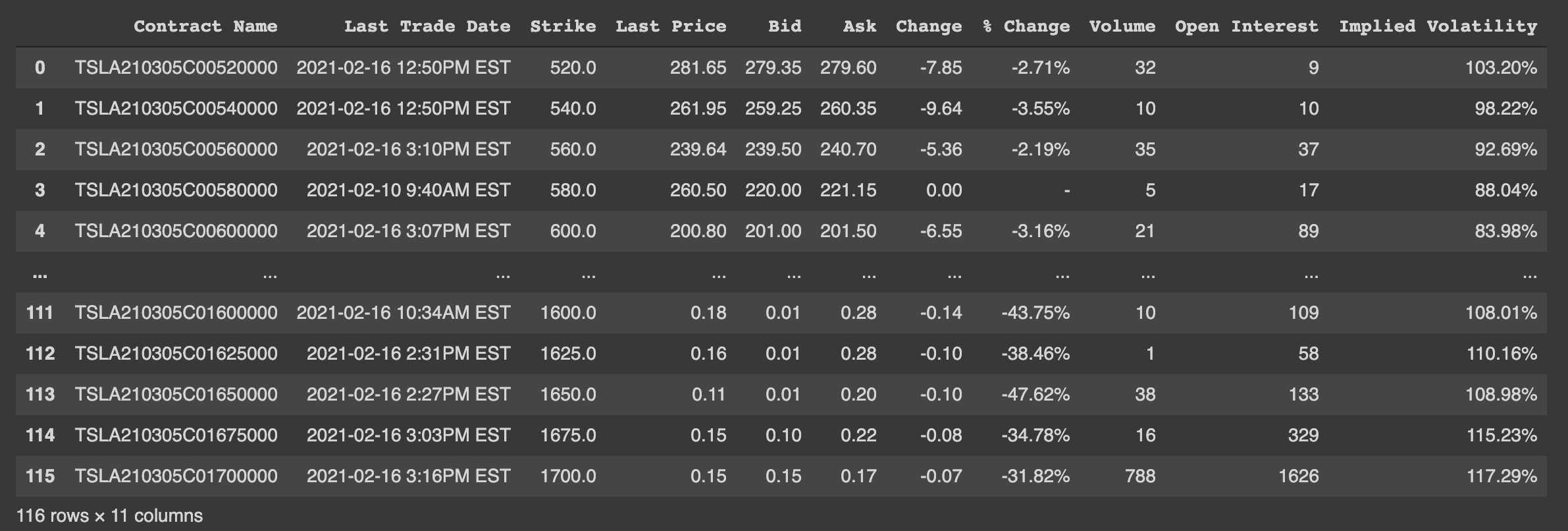
Process Data

We want to remove some outliers by filtering out the options which has very low volumne or open interest.

def remove_outlier(df: pd.DataFrame, current_price: float = None):
  """Some price of option are outlier and need to remove"""
  # df = df.loc[(df["Change"] > 0.001) | (df["Change"] < -0.001)]
  df = df.loc[df["Volume"] != "-"]
  df["Volume"] = df["Volume"].astype(int)
  df["Open Interest"] = df["Open Interest"].astype(int)
  minimum_volume = (df["Volume"] + df["Open Interest"]).quantile(0.1)
  return df.loc[(df["Volume"] + df["Open Interest"]) > minimum_volume]

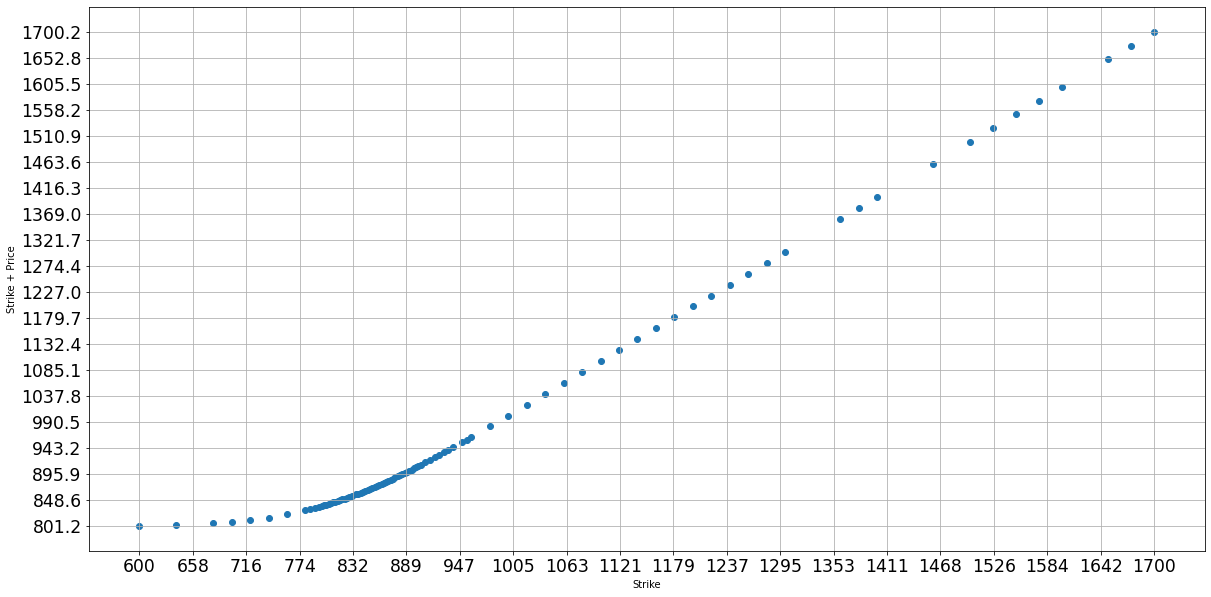
Then let us plot the curve of strike price vs break-even price (strike price + option price):

def plot_strike_profit(df: pd.DataFrame):
  """Plot the strick price vs profit price (strick + cost)"""
  strike = df["Strike"]
  profit = strike + 0.5 * (df["Bid"] + df["Ask"])
  figure = plt.scatter(strike, profit)
  plt.ylabel("Strike + Price")
  plt.xlabel("Strike")
  xticks = np.linspace(np.min(strike), np.max(strike), 20)
  yticks = np.linspace(np.min(profit), np.max(profit), 20)
  plt.xticks(xticks, fontsize="xx-large")
  plt.yticks(yticks, fontsize="xx-large")
  plt.grid(True)
  return figure

Here we use 0.5 * (df["Bid"] + df["Ask"]) for the option price, as it is more stable than Last Price. This is the plot:

Or we could plot strike price vs option extrinsic value:

def plot_strike_extrinsic(df: pd.DataFrame, current_price: float, call_or_put: bool):
  """Plot the strick price vs extrinsic value

  Args:
    df: option data
    current_price: current price of stock
    call_or_put: if True, this is call option
  """
  strike = df["Strike"]
  # extrinsic = price of option if out of money or price of option - abs(strick - current_price)
  if call_or_put:
    extrinsic = 0.5 * (df["Bid"] + df["Ask"]) - np.maximum(0.0, current_price - df["Strike"])
  figure = plt.scatter(strike, extrinsic)
  plt.ylabel("extrinsic")
  plt.xlabel("Strike")
  xticks = np.linspace(np.min(strike), np.max(strike), 20)
  yticks = np.linspace(np.min(extrinsic), np.max(extrinsic), 20)
  plt.xticks(xticks, fontsize="xx-large")
  plt.yticks(yticks, fontsize="xx-large")
  plt.grid(True)
  return figure

This plot matches the Black Scholes Model described in my previous post.

Some Useless Analysis

I also tried whether I could fit some lines to the curve of strike price vs break-even price.

Here is the code.

def fit_line_ransac(x: np.ndarray, y: np.ndarray, error_threshold: float = 1e-3, convergence: float =  0.9, max_iterations: int = 10, initial_sample_size=10):
  """Fit line via ransac"""
  number_data = np.prod(x.shape)
  sample_size = initial_sample_size
  best_quality = 0.0
  best_line = None
  for i in range(max_iterations):
    # random sample the points as initial seed
    sampled_indices = np.random.choice(number_data, sample_size)
    last_quality = 0.0
    while True:
      # fit a curve and find how many points lands on this curve
      line = np.polyfit(x[sampled_indices], y[sampled_indices], 1)
      error = np.abs(y - (line[0] * x + line[1])) / (np.abs(y) + 1e-3)
      sampled_indices = np.where(error <= error_threshold)[0]
      fit_quality = np.sum(error <= error_threshold) / number_data
      if fit_quality - last_quality <= 1e-3:
        # no more new points fitted to this curve
        break
      if sampled_indices.shape[0] < initial_sample_size:
        # too less points lands on the curve
        break
      # refine the curve with all the points on this curve for robustness
      last_quality = fit_quality
    # print(f"Fit result at {i} iterations: {fit_quality * 100}% of data points fits to {line}")
    if last_quality > best_quality:
      best_line = line
      best_quality = last_quality
    # if most points fit to this curve, then we have found a good curve
    # otherwise, try with a new random seed
    if fit_quality >= convergence:
      break
  print(f"Best result: {best_quality * 100}% of data points fits to {best_line}")
  return line

def detect_ankle_point(df: pd.DataFrame, current_price: float = None, error_threshold: float = 1e-3):
  """Fit two linear curve and find where it intersects"""
  plot_strike_profit(df)
  number_data = len(df)
  strike = np.array(df["Strike"])
  profit = np.array(df["Strike"] + 0.5 * (df["Bid"] + df["Ask"]))

  # first curve for bottom 25% of points
  if current_price is None:
    x = strike[:number_data // 4]
    y = profit[:number_data // 4]
  else:
    x = strike[strike <= current_price * 0.9]
    y = profit[strike <= current_price * 0.9]
  line1 = fit_line_ransac(x, y, error_threshold=error_threshold)
  x = strike[[0, -1]]
  y = line1[0] * x + line1[1]
  plt.plot(x, y, color="r", linewidth=2)

  # second curve for top 25% of points
  if current_price is None:
    x = strike[-(number_data // 4):]
    y = profit[-(number_data // 4):]
  else:
    x = strike[strike >= current_price * 1.1]
    y = profit[strike >= current_price * 1.1]
  line2 = fit_line_ransac(x, y, error_threshold=error_threshold)
  x = strike[[0, -1]]
  y = line2[0] * x + line2[1]
  plt.plot(x, y, color="g", linewidth=2)

  # find the intersection
  x = (line2[1] - line1[1]) / (line1[0] - line2[0])
  y = line1[0] * x + line1[1]
  plt.annotate(f"{x:.0f}, {y:.0f}", (x, y), fontsize="xx-large")

  # change axis
  plt.xlim(strike[[0, -1]] * np.asarray([0.95, 1.05]))
  plt.ylim(profit[[0, -1]] * np.asarray([0.95, 1.05]))
  plt.legend([
    f"{line1[0]} * strick + {line1[1]}",
    f"{line2[0]} * strick + {line2[1]}",
    "Strike vs Strick + Price",
  ], fontsize="xx-large")
  return line1, line2, (x, y)

Written on February 16, 2021