XGBoost
[gradient-boosting boosting random-forest decision-tree bagging XGBoost stands for “Extreme Gradient Boosting”, where the term “Gradient Boosting” originates from the paper Greedy Function Approximation: A Gradient Boosting Machine, by Friedman.
The benefits of XGBoost:
- Flexible: Supports regression, classification, ranking and user defined objectives.
- Portable: Runs on Windows, Linux and OS X, as well as various cloud Platforms.
- Multiple Languages: Supports multiple languages including C++, Python, R, Java, Scala, Julia.
- Battle-tested: Wins many data science and machine learning challenges. Used in production by multiple companies.
- Distributed on Cloud: Supports distributed training on multiple machines, including AWS, GCE, Azure, and Yarn clusters. Can be integrated with Flink, Spark and other cloud dataflow systems.
- Performance: The well-optimized backend system for the best performance with limited resources. The distributed version solves problems beyond billions of examples with same code.
Classification and Regression Trees (CART)
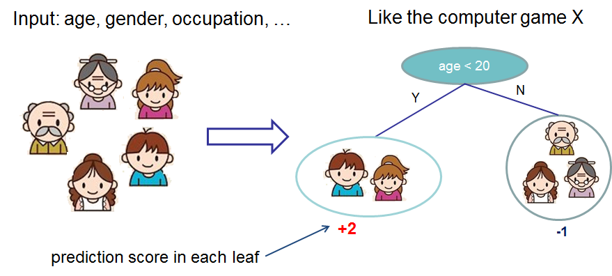
We classify the members of a family into different leaves, and assign them the score on the corresponding leaf. A CART is a bit different from decision trees, in which the leaf only contains decision values. In CART, a real score is associated with each of the leaves, which gives us richer interpretations that go beyond classification.
Random Forest
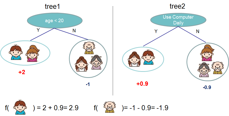
Usually, a single tree is not strong enough to be used in practice. What is actually used is the ensemble model, which sums the prediction of multiple trees together.
The objective function is written as:
\(\ell(\theta)=\sum_i{\ell(y_i - \hat{y}_i)+\sum_k{\Omega(f_k)}}\) where $\hat{y}_i=\sum_k{f_k(x_i)}$ is the prediction.
Gradient Bossting
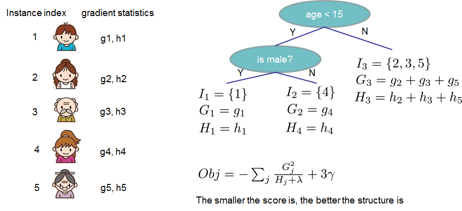
The first question we want to ask: what are the parameters of trees? You can find that what we need to learn the structure of the tree and the leaf scores. Learning tree structure is much harder than traditional optimization problem where you can simply take the gradient. It is intractable to learn all the trees at once. Instead, we use an additive strategy: fix what we have learned, and add one new tree at a time.
\[\hat{y}_i^t=\sum_k^t{f_k{x_i}}=\hat{y}_i^{t-1}+f_t(x_i)\]By applying thre gradient, we will have:
\[\sum_i{[g_if_t(x_i)+\frac{1}{2}h_if_t(x_i)]}+\Omega(f_t)\\ g_i=\frac{\partial \ell(y_i,\hat{y}_i^{t-1})}{\partial \hat{y}_i^{t-1}}\\ h_i=\frac{\partial \ell(y_i,\hat{y}_i^{t-1})}{\partial^2 \hat{y}_i^{t-1}}\]