Elucidating the Design Space of Diffusion-Based Generative Models
[diffusion dppm deep-learning fid ddim ode This is my reading note for Elucidating the Design Space of Diffusion-Based Generative Models. This paper checks the varying design of diffusion method and proposed a unify frame work to incorporate them. Finally the author proposes optimal choice of diffusion method under this frame work.
Introduction
We argue that the theory and practice of diffusion-based generative models are currently unnecessarily convoluted and seek to remedy the situation by presenting a design space that clearly separates the concrete design choices. This lets us identify several changes to both the sampling and training processes, as well as preconditioning of the score networks (p. 1)
Expressing diffusion models in a common framework
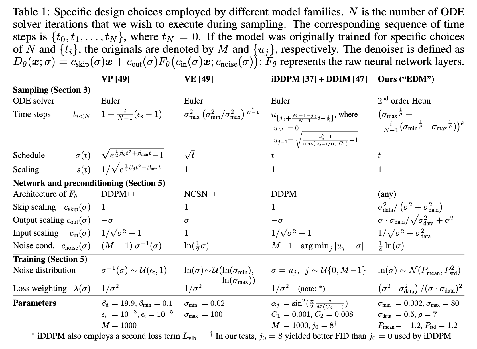
Let us denote the data distribution by $p_{data}(x)$, with standard deviation $\sigma_{data}$, and consider the family of mollified distributions $p(x; \sigma)$ obtained by adding i.i.d. Gaussian noise of standard deviation $\sigma$ to the data. For $\sigma_{max}$ and $\sigma_{data}$, $p(x; \sigma_{max})$ is practically indistinguishable from pure Gaussian noise. The idea of diffusion models is to randomly sample a noise image $x_0 \approx N (0, \sigma^2{max} I)$, and sequentially denoise it into images xi with noise levels $\sigma_0 = \sigma{max} > \sigma_1 > \cdots > \sigma_N = 0$ so that at each noise level $x_i \approx p(x_i; \sigma_i)$. The endpoint $x_N$ of this process is thus distributed according to the data (p. 2)
ODE formulation. A probability flow ODE [49] continuously increases or reduces noise level of the image when moving forward or backward in time, respectively. To specify the ODE, we must first choose a schedule σ(t) that defines the desired noise level at time t. For example, setting $\sigma(t) \propto\sqrt{t}$ is mathematically natural, as it corresponds to constant-speed heat diffusion [12]. However, we will show in Section 3 that the choice of schedule has major practical implications and should not be made on the basis of theoretical convenience (p. 2)
Improvements to deterministic sampling
Our hypothesis is that the choices related to the sampling process are largely independent of the other components, such as network architecture and training details (p. 4)
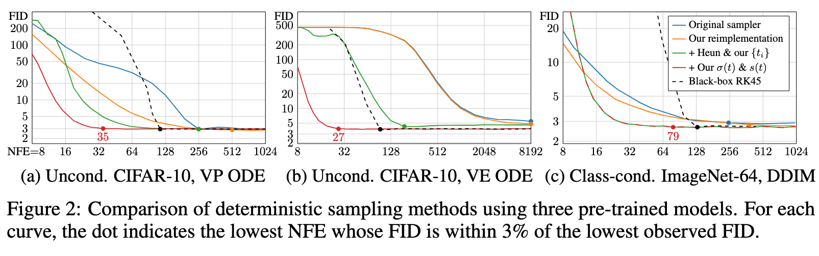
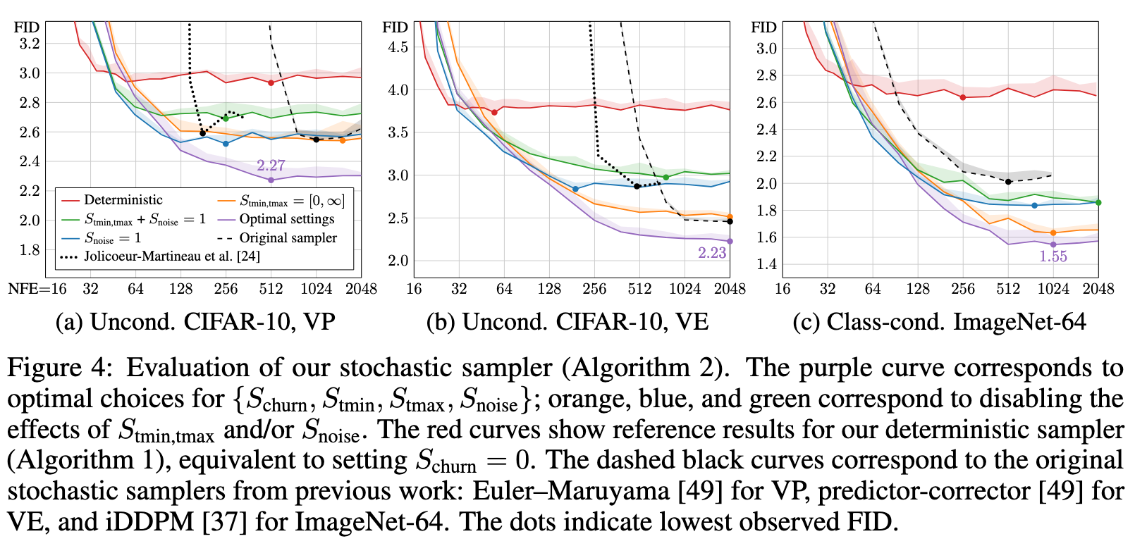
The original deterministic samplers are shown in blue, and the reimple- mentations of these methods in our unified framework (orange) yield similar but consistently better results. The differences are explained by certain oversights in the original implementations as well as our more careful treatment of discrete noise levels in the case of DDIM (p. 4)
Solving an ODE numerically is necessarily an approximation of following the true solution trajectory. At each step, the solver introduces truncation error that accumulates over the course of N steps. The local error generally scales superlinearly with respect to step size, and thus increasing N improves the accuracy of the solution. (p. 4)
The commonly used Euler’s method is a first order ODE solver with O(h2) local error with respect to step size h. Higher-order Runge–Kutta methods [50] scale more favorably but require multiple (p. 4)evaluations of Dθ per step. Linear multistep methods have also been recently proposed for sampling diffusion models [31, 59]. Through extensive tests, we have found Heun’s 2nd order method [2] (a.k.a. improved Euler, trapezoidal rule) — previously explored in the context of diffusion models by Jolicoeur-Martineau et al. [24] — to provide an excellent tradeoff between truncation error and NFE.
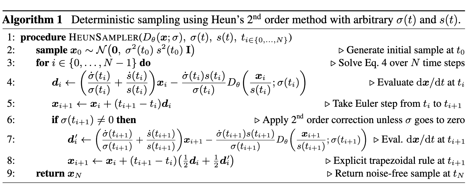
As illustrated in Algorithm 1, it introduces an additional correction step for xi+1 to account for change in dx/dt between ti and ti+1. This correction leads to O(h3) local error at the cost of one additional evaluation of Dθ per step. Note that stepping to σ = 0 would result in a division by zero, so we revert to Euler’s method in this case. (p. 5)
We provide a detailed analysis in Appendix D.1, concluding that the step size should decrease monotonically with decreasing σ and it does not need to vary on a per-sample basis. (p. 5)

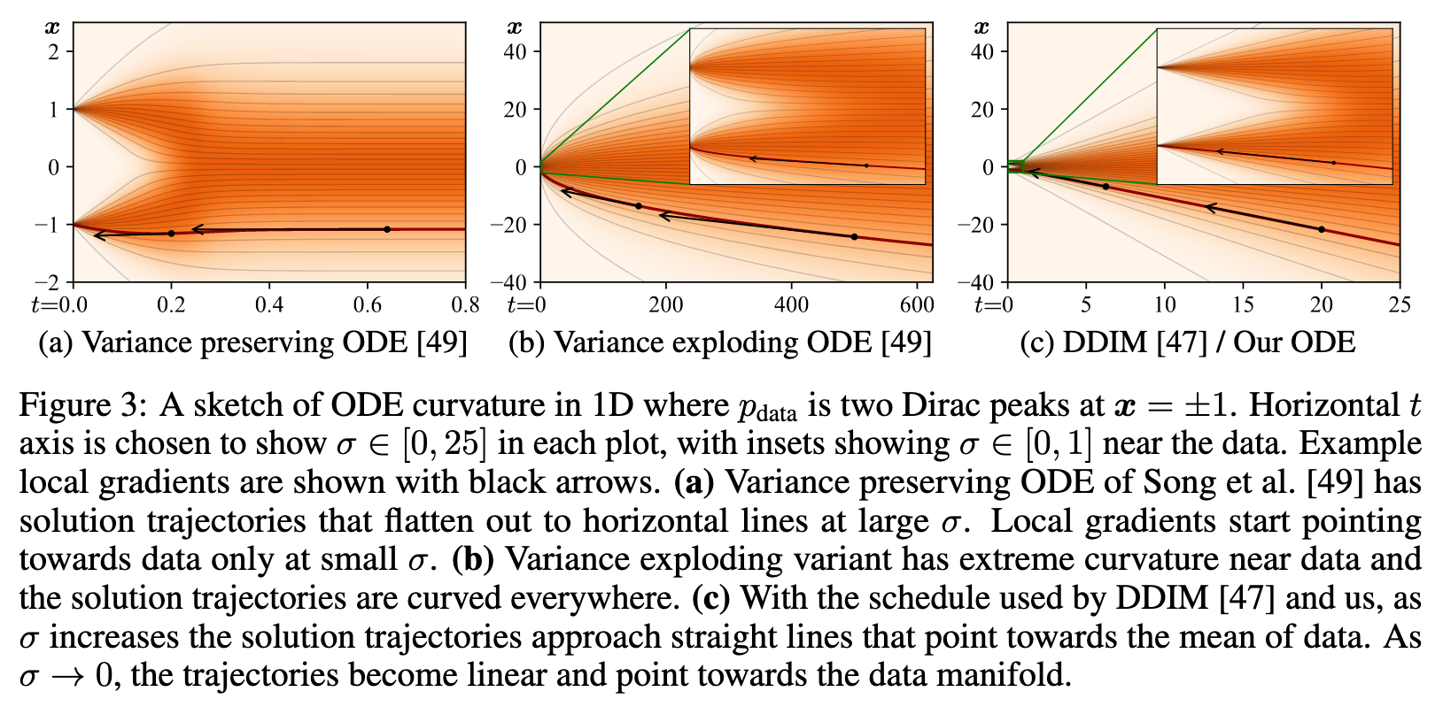
Trajectory curvature and noise schedule. The shape of the ODE solution trajectories is defined by functions σ(t) and s(t). The choice of these functions offers a way to reduce the truncation errors discussed above, as their magnitude can be expected to scale proportional to the curvature of $\frac{d_x}{d_t}$.
We argue that the best choice for these functions is $\sigma(t)$ = t and $s(t) = 1$, which is also the choice made in DDIM [47]. With this choice, the ODE of Eq. 4 simplifies to $\frac{d_x}{d_t} = x − \frac{D(x;t)}{t}$ and σ and t become interchangeable. (p. 5)
Stochastic sampling
Deterministic sampling offers many benefits, e.g., the ability to turn real images into their corresponding latent representations by inverting the ODE. However, it tends to lead to worse output quality [47, 49] than stochastic sampling that injects fresh noise into the image in each step. Given that ODEs and SDEs recover the same distributions in theory, what exactly is the role of stochasticity? Background. The SDEs of Song et al. [49] can be generalized [20, 58] as a sum of the probability flow ODE of Eq. 1 and a time-varying Langevin diffusion SDE [14] (see Appendix B.5): (p. 6)
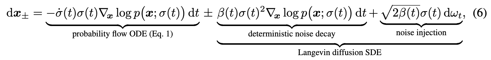
where $\omega_t$ is the standard Wiener process. $dx_+$ and $dx_−$ are now separate SDEs for moving forward and backward in time, related by the time reversal formula of Anderson [1]. The Langevin term can further be seen as a combination of a deterministic score-based denoising term and a stochastic noise injection term, whose net noise level contributions cancel out. As such, β(t) effectively expresses the relative rate at which existing noise is replaced with new noise. The SDEs of Song et al. [49] are recovered with the choice $\beta(t) = \dot{\sigma}(t)/\sigma(t)$, whereby the score vanishes from the forward SDE.
This perspective reveals why stochasticity is helpful in practice: The implicit Langevin diffusion drives the sample towards the desired marginal distribution at a given time, actively correcting for any errors made in earlier sampling steps. On the other hand, approximating the Langevin term with discrete SDE solver steps introduces error in itself. Previous results [3, 24, 47, 49] suggest that non-zero β(t) is helpful, but as far as we can tell, the implicit choice for β(t) in Song et al. [49] enjoys no special properties. Hence, the optimal amount of stochasticity should be determined empirically. (p. 6)
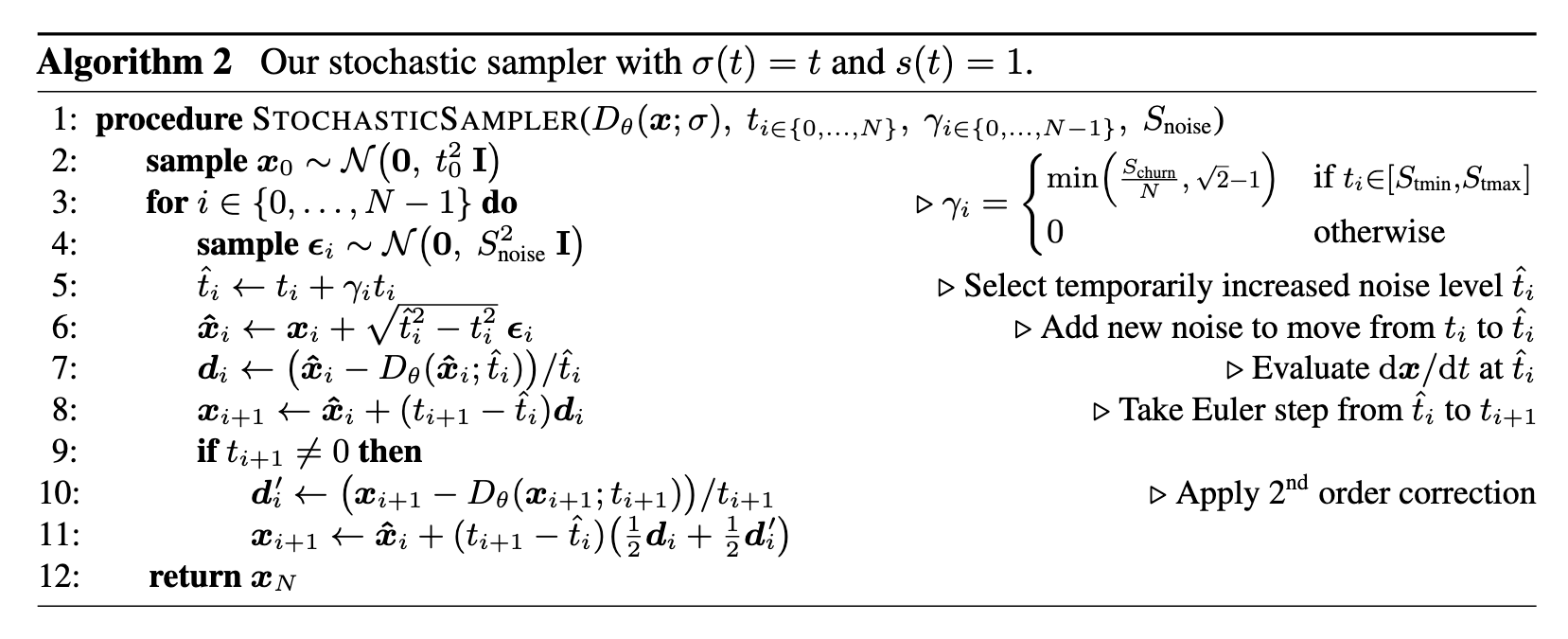
Add new noise to move from ti to tˆi (p. 7)
One can interpret Euler–Maruyama as first adding noise and then performing an ODE step, not from the intermediate state after noise injection, but assuming that x and σ remained at the initial state at the beginning of the iteration step. In our method, the parameters used to evaluate Dθ on line 7 of Algorithm 2 correspond to the state after noise injection (p. 7)
Practical considerations. Increasing the amount of stochasticity is effective in correcting errors made by earlier sampling steps, but it has its own drawbacks. We have observed (see Appendix E.1) that excessive Langevin-like addition and removal of noise results in gradual loss of detail in the generated images with all datasets and denoiser networks. There is also a drift toward oversaturated colors at very low and high noise levels. We suspect that practical denoisers induce a slightly non- conservative vector field in Eq. 3, violating the premises of Langevin diffusion and causing these detrimental effects. Notably, our experiments with analytical denoisers (such as the one in Figure 1b) have not shown such degradation. (p. 7)
We address the drift toward oversaturated colors by only enabling stochasticity within a specific range of noise levels $t_i \in [S_{tmin}, S_{tmax}]$. For these noise levels, we define $\gamma_i = S_{churn}/N$, where S churn controls the overall amount of stochasticity. We further clamp $\gamma_i$ to never introduce more new noise than what is already present in the image. Finally, we have found that the loss of detail can be partially counteracted by setting S noise slightly above 1 to inflate the standard deviation for the newly added noise. This suggests that a major component of the hypothesized non-conservativity of $D_\theta(x; \sigma)$ is a tendency to remove slightly too much noise — most likely due to regression toward the mean that can be expected to happen with any L2-trained denoiser (p. 7)
Further results with stochastic sampling
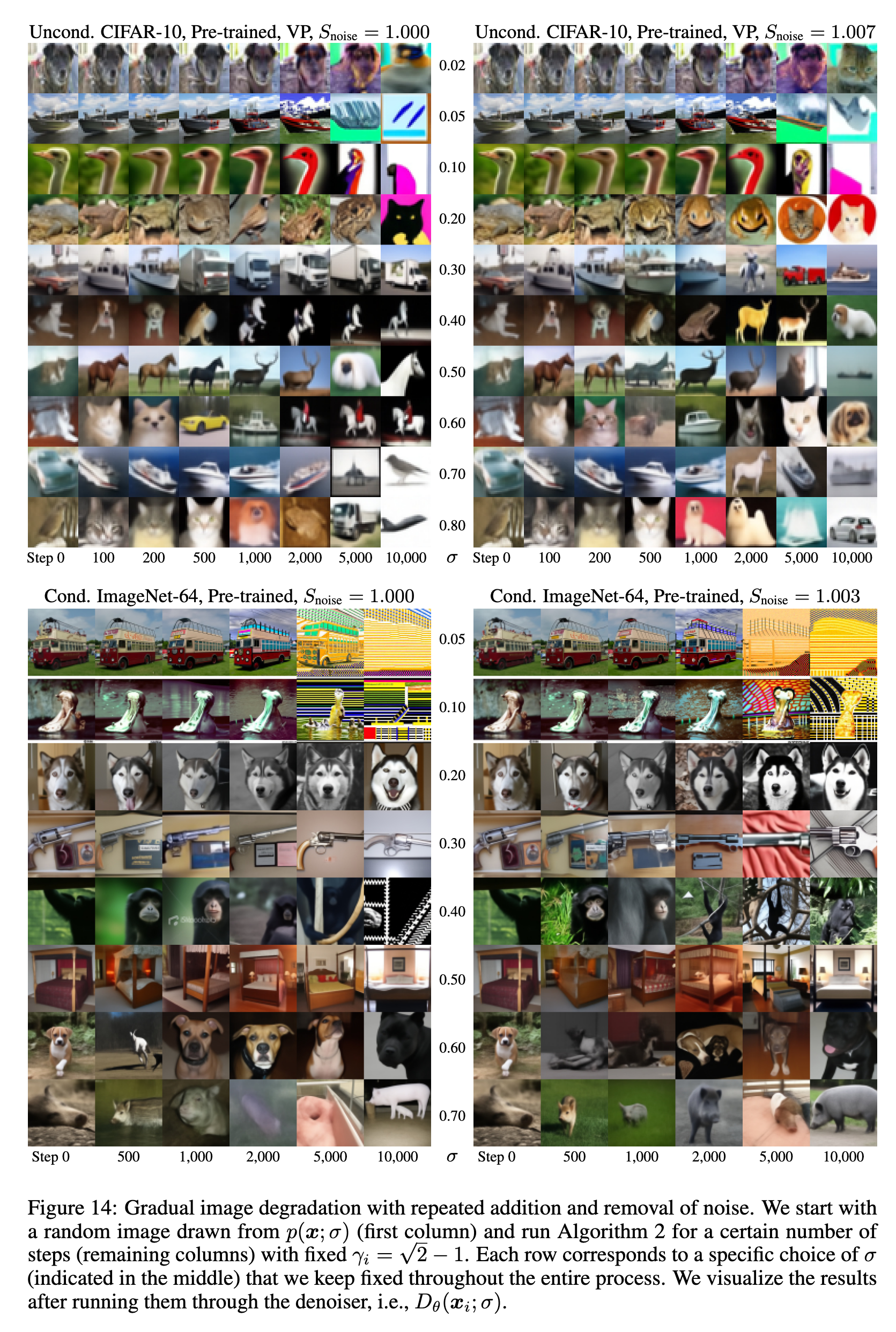
Figure 14 illustrates the image degradation caused by excessive Langevin iteration (Section 4, “Practical considerations”). These images are generated by doing a specified number of iterations at a fixed noise level σ so that at each iteration an equal amount of noise is added and removed. In theory, Langevin dynamics should bring the distribution towards the ideal distribution p(x; σ) but as noted in Section 4, this holds only if the denoiser $ = x − \sigma F_{\theta}(\dot )$ induces a conservative vector field in Eq. 3. (p. 41)
As seen in the figure, it is clear that the image distribution suffers from repeated iteration in all cases, although the exact failure mode depends on dataset and noise level. For low noise levels (below 0.2 or so), the images tend to oversaturate starting at 2k iterations and become fully corrupted after that. Our heuristic of setting S_tmin > 0 is designed to prevent stochastic sampling altogether at very low noise levels to avoid this effect.
For high noise levels, we can see that iterating without the standard deviation correction, i.e., when Snoise = 1.000, the images tend to become more abstract and devoid of color at high iteration counts; this is especially visible in the 10k column of CIFAR-10 where the images become mostly black and white with no discernible backgrounds. Our heuristic inflation of standard deviation by setting Snoise > 1 counteracts this tendency efficiently, as seen in the corresponding images on the right hand side of the figure. Notably, this still does not fix the oversaturation and corruption at low noise levels, suggesting multiple sources for the detrimental effects of excessive iteration. Further research will be required to better understand the root causes of these observed effects. (p. 41)
Preconditioning and training
There are various known good practices for training neural networks in a supervised fashion. For example, it is advisable to keep input and output signal magnitudes fixed to, e.g., unit variance, and to avoid large variation in gradient magnitudes on a per-sample basis [5, 21]. Training a neural network to model D directly would be far from ideal — for example, as the input x = y + n is a combination of clean signal y and noise $n ∼ N (0, \sigma^2 I)$, its magnitude varies immensely depending on noise level σ. For this reason, the common practice is to not represent $D_\theta$ as a neural network directly, but instead train a different network $F_\theta$ from which $D_\theta$ is derived. (p. 8)
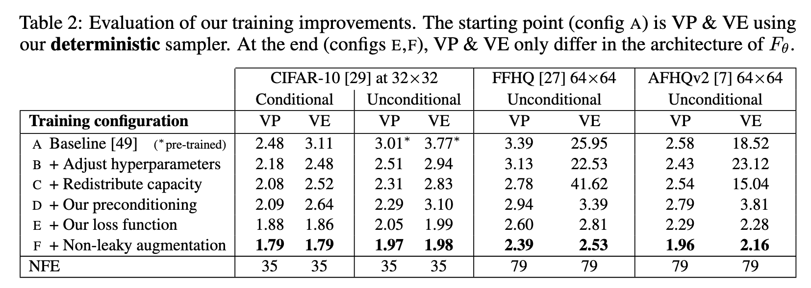
Previous methods [37, 47, 49] address the input scaling via a σ-dependent normalization factor and attempt to precondition the output by training Fθ to predict n scaled to unit variance, from which the signal is then reconstructed via $D_\theta(x; \sigma) = x − \sigma F_{\theta}(\dot )$. This has the drawback that at large σ, the network needs to fine-tune its output carefully to cancel out the existing noise n exactly and give the output at the correct scale; note that any errors made by the network are amplified by a factor of σ. In this situation, it would seem much easier to predict the expected output $D_\theta(x; \sigma)$ directly. (p. 8) This is also shown in Table 2, where preconditioning doesn’t help for most of the time.


Loss weighting and sampling. Inspecting the per-σ loss after training (blue and orange curves) reveals that a significant reduction is possible only at intermediate noise levels; at very low levels, it is both difficult and irrelevant to discern the vanishingly small noise component, whereas at high levels the training targets are always dissimilar from the correct answer that approaches dataset average. Therefore, we target the training efforts to the relevant range using a simple log-normal distribution for ptrain(σ) as detailed in Table 1 and illustrated in Figure 5a (red curve). (p. 9)
Augmentation regularization. To prevent potential overfitting that often plagues diffusion models with smaller datasets, we borrow an augmentation pipeline from the GAN literature [25]. The pipeline consists of various geometric transformations (see Appendix F.2) that we apply to a training image prior to adding noise. To prevent the augmentations from leaking to the generated images, we provide the augmentation parameters as a conditioning input to Fθ; during inference we set the them to zero to guarantee that only non-augmented images are generated. (p. 9)