Billion-scale similarity search with GPUs
[knn database llm kmeans vector sort quantization faiss This is my reading note on Billion-scale similarity search with GPUs. FAISS (Facebook AI Similarity Search) is an open-source library that allows developers to quickly search for similar embeddings of multimedia documents. FAISS uses indexing structures like LSH, IVF, and PQ to speed up the search. It also supports GPUs, which can further accelerate the search. FAISS was developed by Facebook AI Research (FAIR).
Introduction
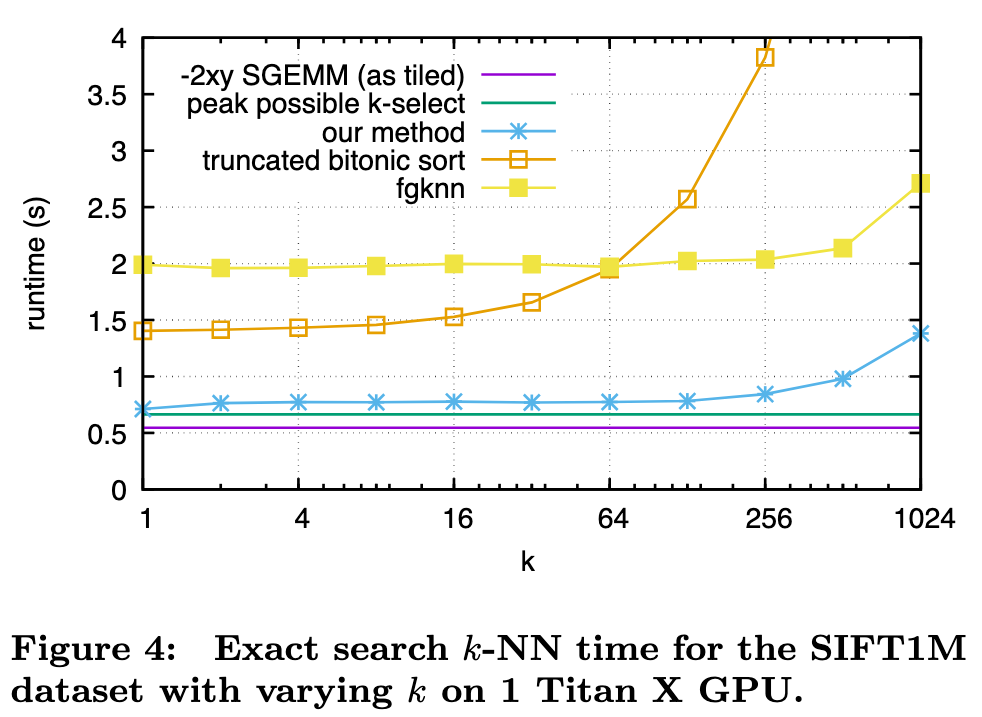
This paper tackles the problem of better utilizing GPUs for this task. While GPUs excel at data-parallel tasks, prior approaches are bottlenecked by algorithms that expose less parallelism, such as k-min selection, or make poor use of the memory hierarchy. We propose a design for k-selection that operates at up to 55% of theoretical peak performance, enabling a nearest neighbor implementation that is 8.5× faster than prior GPU state of the art. (p. 1)
Note, state of the art methods like NN-Descent [15] have a large memory overhead on top of the dataset itself and cannot readily scale to the billion-sized databases we consider. (p. 1)
Such applications must deal with the curse of dimensionality [46], rendering both exhaustive search or exact indexing for non-exhaustive search impractical on billion-scale databases. This is why there is a large body of work on approximate search and/or graph construction. To handle huge datasets that do not fit in RAM, several approaches employ an internal compressed representation of the vectors using an encoding. This is especially convenient for memory-limited devices like GPUs. It turns out that accepting a minimal accuracy loss results in orders of magnitude of compression [21]. The most popular vector compression methods can be classified into either binary codes [18, 22], or quantization methods [25, 37]. Both have the desirable property that searching neighbors does not require reconstructing the vectors. (p. 1)
Our paper focuses on methods based on product quantization (PQ) codes, as these were shown to be more effective than binary codes [34]. In addition, binary codes incur important overheads for non-exhaustive search methods [35]. Several improvements were proposed after the original product quantization proposal known as IVFADC [25]; most are difficult to implement efficiently on GPU. For instance, the inverted multi-index [4], useful for high-speed/low-quality operating points, depends on a complicated “multi-sequence” algorithm. The optimized product quantization or OPQ [17] is a linear transformation on the input vectors that improves the accuracy of the product quantization; it can be applied as a pre-processing. The SIMD-optimized IVFADC implementation from [2] operates only with sub-optimal parameters (few coarse quantization centroids). Many other methods, like LOPQ and the Polysemous codes [27, 16] are too complex to be implemented efficiently on GPUs. (p. 2)
PROBLEM STATEMENT
Exact search
The exact solution computes the full pairwise distance matrix $D=\lVert x_j y_i\rVert_2^2 \in \mathbb{R}^{n_q times l}$. In practice, we use the decomposition (p. 2)
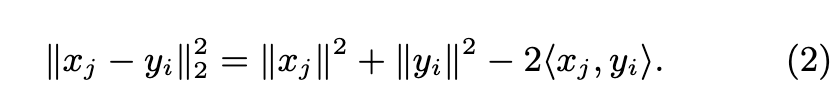
The two first terms can be precomputed in one pass over the matrices X and Y whose rows are the [xj ] and [yi]. The bottleneck is to evaluate hxj , yii, equivalent to the matrix multiplication XY >. The k-nearest neighbors for each of the nq queries are k-selected along each row of D. (p. 2)
Compressed-domain search
From now on, we focus on approximate nearest-neighbor search. We consider, in particular, the IVFADC indexing structure [25]. The IVFADC index relies on two levels of quantization, and the database vectors are encoded. The database vector y is approximated as: (p. 2)
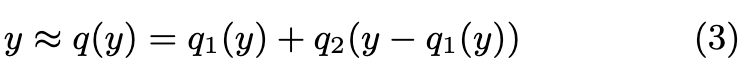
Since the sets are finite, q(y) is encoded as the index of q1(y) and that of q2(y −q1(y)). The first-level quantizer is a coarse quantizer and the second level fine quantizer encodes the residual vector after the first level. (p. 2)
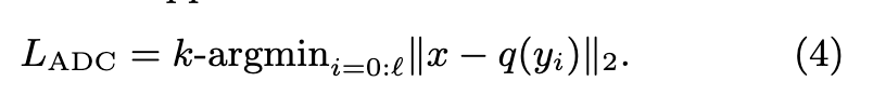
For IVFADC the search is not exhaustive. Vectors for which the distance is computed are pre-selected depending on the first-level quantizer q1 (p. 2)
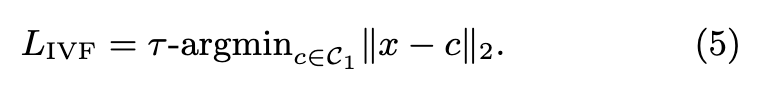
The multi-probe parameter τ is the number of coarse-level centroids we consider. The quantizer operates a nearestneighbor search with exact distances, in the set of reproduction values. Then, the IVFADC search computes (p. 2)
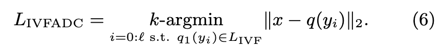
| The corresponding data structure, the inverted file, groups the vectors yi into | C1 | inverted lists I1, …, I | C1 | with homogeneous q1(yi). Therefore, the most memory-intensive operation is computing LIVFADC, and boils down to linearly scanning τ inverted lists. (p. 2) |
The quantizers
The quantizers q1 and q2 have different properties. q1 needs to have a relatively low number of reproduction values so that the number of inverted lists does not explode. We typically use |C1| ≈ √`, trained via k-means. For q2, we can afford to spend more memory for a more extensive representation. The ID of the vector (a 4or 8-byte integer) is also stored in the inverted lists, so it makes no sense to have shorter codes than that; i.e., log2 |C2| > 4 × 8. (p. 2)
Product quantizer
We use a product quantizer [25] for q2, which provides a large number of reproduction values without increasing the processing cost. It interprets the vector y as b sub-vectors y = [y0…yb−1], where b is an even divisor of the dimension d. Each sub-vector is quantized with its own quantizer, yielding the tuple (q0(y0), …, qb−1(yb−1)). The sub-quantizers typically have 256 reproduction values, to fit in one byte. The quantization value of the product quantizer is then q2(y) = q0(y0) + 256 × q1(y1) + … + 256b−1 × qb−1 , which from a storage point of view is just the concatenation of the bytes produced by each sub-quantizer. (p. 3)
GPU: OVERVIEW AND K-SELECTION
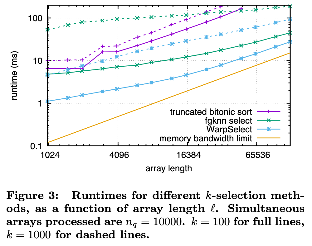
k-selection algorithms, often for arbitrarily large l and k, can be translated to a GPU, including radix selection and bucket selection [1], probabilistic selection [33], quickselect [14], and truncated sorts [40]. Their performance is dominated by multiple passes over the input in global memory. (p. 3)
In-register sorting
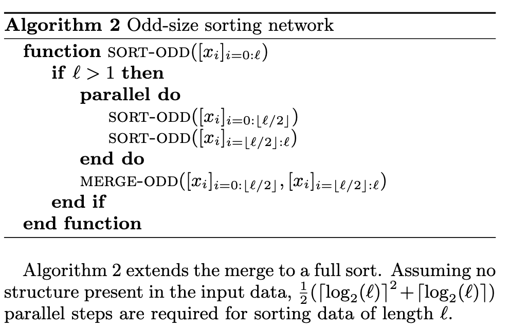
We use an in-register sorting primitive as a building block. Sorting networks are commonly used on SIMD architectures [13], as they exploit vector parallelism. They are easily implemented on the GPU, and we build sorting networks with lane-stride register arrays. (p. 4)
We use a variant of Batcher’s bitonic sorting network [8], which is a set of parallel merges on an array of size 2k. Each merge takes s arrays of length t (s and t a power of 2) to s/2 arrays of length 2t, using log2(t) parallel steps. A bitonic sort applies this merge recursively (p. 4)
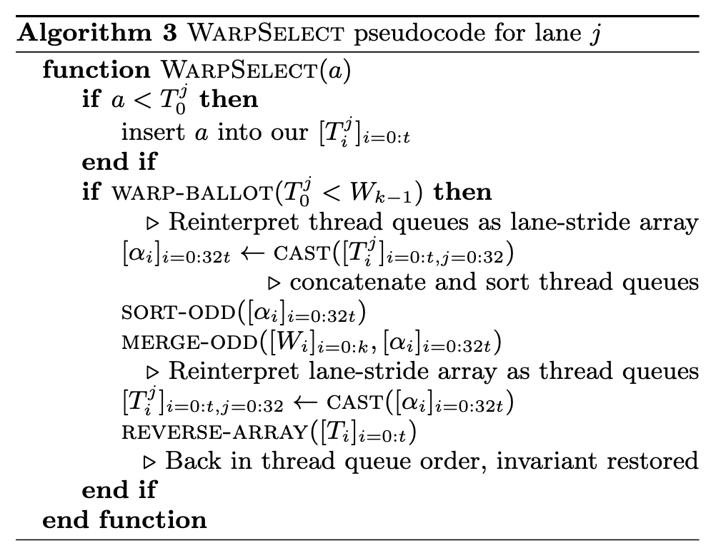
WarpSelect
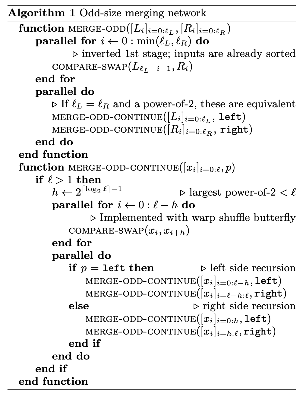
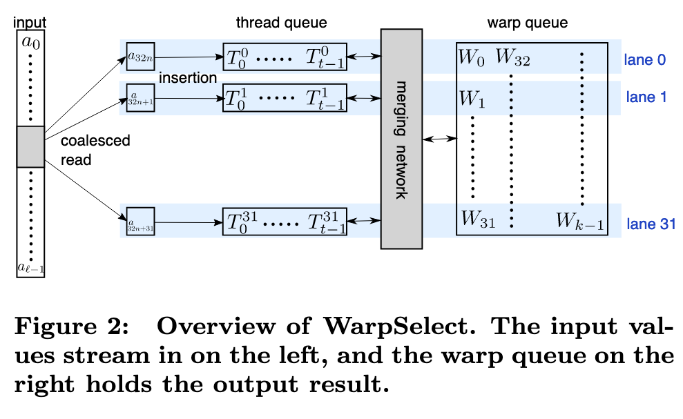
Our k-selection implementation, WarpSelect, maintains state entirely in registers, requires only a single pass over data and avoids cross-warp synchronization. It uses mergeodd and sort-odd as primitives. Since the register file provides much more storage than shared memory, it supports k ≤ 1024. Each warp is dedicated to k-selection to a single one of the n arrays [ai]. If n is large enough, a single warp per each [ai] will result in full GPU occupancy. Large ` per warp is handled by recursive decomposition, if ` is known in advance (p. 5)
Each lane j maintains a small queue of t elements in registers, called the thread queues [Tj i ]i=0:t, ordered from largest to smallest (Tj i ≥ Tj i+1) (p. 5)
If a new a32i+j is greater than the largest key currently in the queue, Tj 0 , it is guaranteed that it won’t be in the k smallest final results. The warp shares a lane-stride register array of k smallest seen elements, [Wi]i=0:k, called the warp queue. It is ordered from smallest to largest (Wi ≤ Wi+1); if the requested k is not a multiple of 32, we round it up. This is a second level data structure that will be used to maintain all of the k smallest warp-wide seen values. (p. 5)
Update. The three invariants maintained are:
- all per-lane Tj 0 are not in the min-k
- all per-lane Tj 0 are greater than all warp queue keys Wi
- all ai seen so far in the min-k are contained in either some lane’s thread queue ([Tj i ]i=0:t,j=0:32), or in the warp queue. (p. 5)
Lane j receives a new a_32i+j and attempts to insert it into its thread queue. If a_32i+j > Tj 0 , then the new pair is by definition not in the k minimum, and can be rejected. Otherwise, it is inserted into its proper sorted position in the thread queue, thus ejecting the old Tj 0 . All lanes complete doing this with their new received pair and their thread queue, but it is now possible that the second invariant have been violated. Using the warp ballot instruction, we determine if any lane has violated the second invariant. If not, we are free to continue processing new elements. (p. 5)
If any lane has its invariant violated, then the warp uses odd-merge to merge and sort the thread and warp queues together. (p. 5)
Complexity and parameter selection
The practical choice for t given k and l was made by experiment on a variety of k-NN data. For k ≤ 32, we use t = 2, k ≤ 128 uses t = 3, k ≤ 256 uses t = 4, and k ≤ 1024 uses t = 8, all irrespective of l (p. 6)
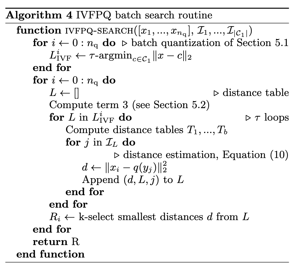
COMPUTATION LAYOUT
-
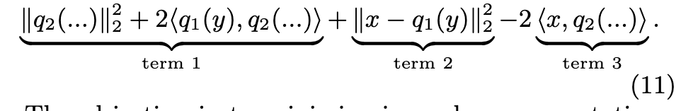
Term 1 is independent of the query. It can be precomputed from the quantizers, and stored in a table T of size C1 × 256 × b; - Term 2 is the distance to q1’s reproduction value. It is thus a by-product of the first-level quantizer q1;
- Term 3 can be computed independently of the inverted list. Its computation costs d × 256 multiply-adds. (p. 7)
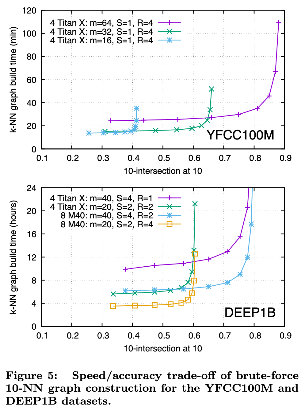
Multi-GPU parallelism
Replication. If an index instance fits in the memory of a single GPU, it can be replicated across R different GPUs. To query nq vectors, each replica handles a fraction nq/R of the queries, joining the results back together on a single GPU or in CPU memory. Replication has near linear speedup, except for a potential loss in efficiency for small nq.
Sharding. If an index instance does not fit in the memory of a single GPU, an index can be sharded across S different GPUs. For adding l vectors, each shard receives l/S of the vectors, and for query, each shard handles the full query set nq, joining the partial results (an additional round of kselection is still required) on a single GPU or in CPU memory. For a given index size l, sharding will yield a speedup (sharding has a query of nq against l/S versus replication with a query of nq/R against l), but is usually less than pure replication due to fixed overhead and cost of subsequent k-selection.
Replication and sharding can be used together (S shards, each with R replicas for S × R GPUs in total). Sharding or replication are both fairly trivial, and the same principle can be used to distribute an index across multiple machines. (p. 7)
Experiments