Large Language Models as Optimizers
[linear-regression optimizer llm deep-learning traveling-salesman-problem tool This is my reading note for Large Language Models as Optimizers. This paper discusses how to prompt larger language model to solve optimization problem, especially how to engineer the prompt to solve the optimization problem. The experiments indicate LLM is capable of solve optimization problem reasonable well, especially when problem is small and starting problem is not far from the final solution.
Introduction
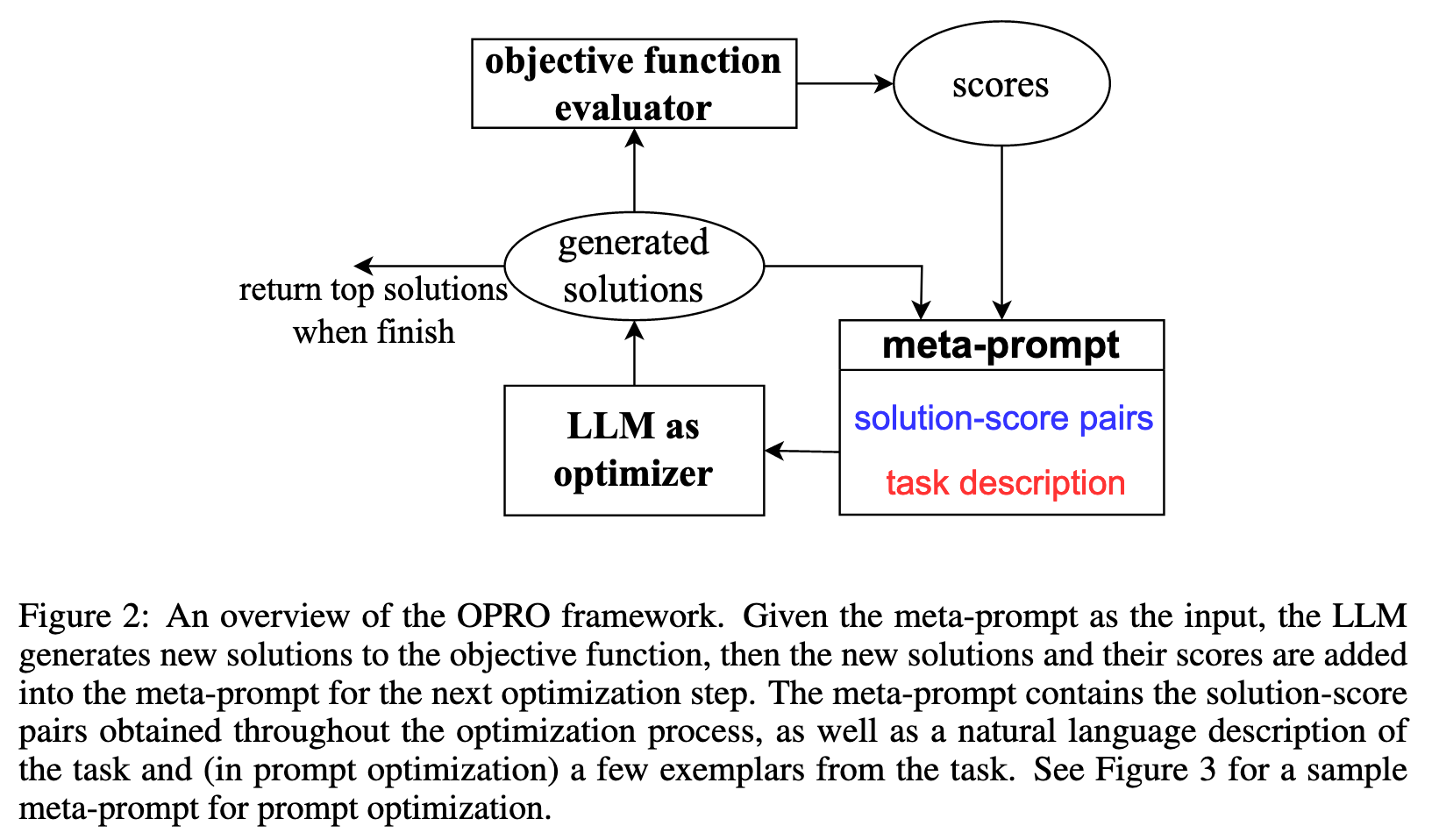
In this work, we propose Optimization by PROmpting (OPRO), a simple and effective approach to leverage large language models (LLMs) as optimizers, where the optimization task is described in natural language. In each optimization step, the LLM generates new solutions from the prompt that contains previously generated solutions with their values, then the new solutions are evaluated and added to the prompt for the next optimization step. (p. 1)
LLMs are shown to be sensitive to the prompt format (Zhao et al., 2021; Lu et al., 2021; Wei et al., 2023; Madaan & Yazdanbakhsh, 2022); in particular, semantically similar prompts may have drastically different performance (Kojima et al., 2022; Zhou et al., 2022b; Zhang et al., 2022), and the optimal prompt formats can be model-specific and task-specific (Ma et al., 2023; Chen et al., 2023c). Therefore, prompt engineering is often important for LLMs to achieve good performance (Reynolds & McDonell, 2021). However, the large and discrete prompt space makes it challenging for optimization, especially when only API access to the LLM is available (p. 2)
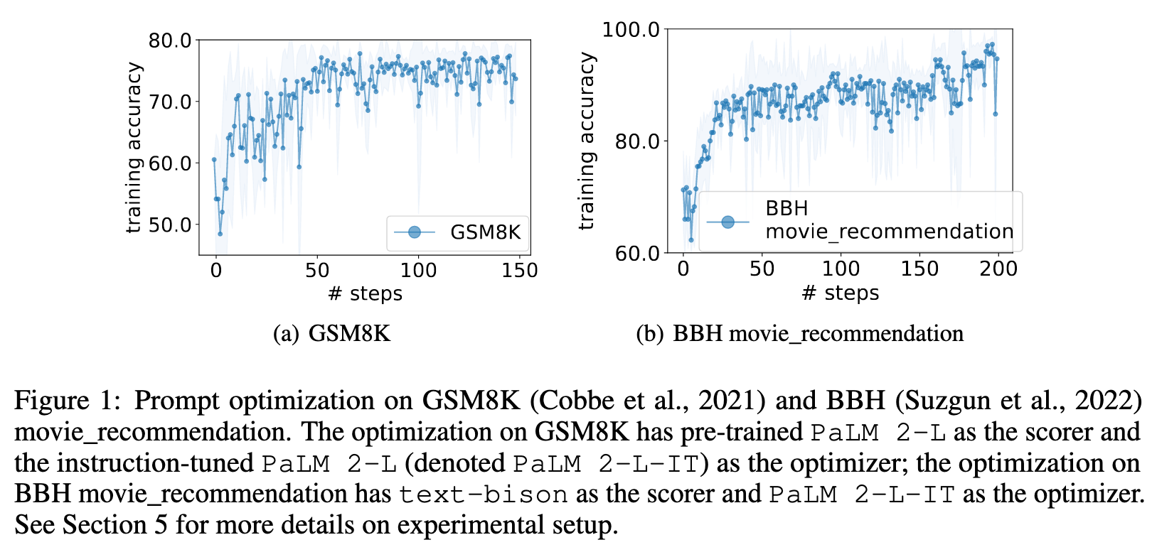
we show in experiments that optimizing the prompt for accuracy on a small training set is sufficient to reach high performance on the test set. (p. 2)
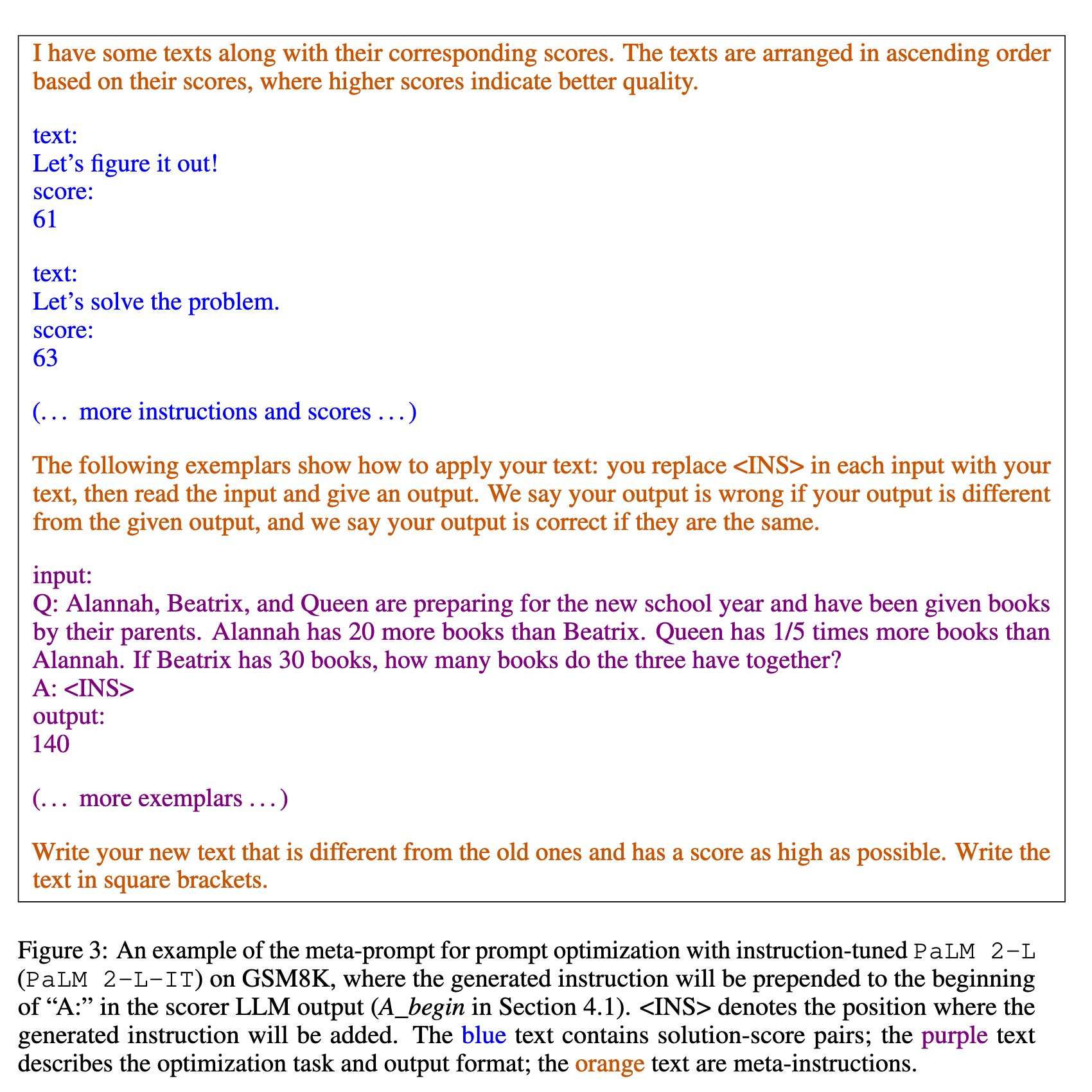
The prompt to the LLM serves as a call to the optimizer, and we name it the meta-prompt. Figure 3 shows an example. The meta-prompt contains two core pieces of information. The first piece is previously generated prompts with their corresponding training accuracies. The second piece is the optimization problem description, which includes several exemplars randomly selected from the training set to exemplify the task of interest. We also provide instructions for the LLM to understand the relationships among different parts and the desired output format. Different from recent work on using LLMs for automatic prompt generation (Zhou et al., 2022b; Pryzant et al., 2023), each optimization step in our work generates new prompts that aim to increase the test accuracy based on a trajectory of previously generated prompts, instead of editing one input prompt according to natural language feedback (Pryzant et al., 2023) or requiring the new prompt to follow the same semantic meaning (Zhou et al., 2022b). Making use of the full optimization trajectory, OPRO enables the LLM to gradually generate new prompts that improve the task accuracy throughout the optimization process, where the initial prompts have low task accuracies. (p. 2)
Proposed Method
META-PROMPT DESIGN
Optimization problem description. The first part is the text description of the optimization problem, including the objective function and solution constraints. For example, for prompt optimization, the LLM can be instructed to “generate a new instruction that achieves a higher accuracy”, and we denote such instructions in the meta-prompt as meta-instructions. We can also provide customized meta-instructions as an informal regularization of the generated solutions, such as “the instruction should be concise and generally applicable”.
Optimization trajectory. Besides understanding natural language instructions, LLMs are also shown to be able to recognize patterns from in-context demonstrations (Wei et al., 2023; Madaan & Yazdanbakhsh, 2022; Mirchandani et al., 2023). Our meta-prompt makes use of this property and instructs the LLM to leverage the optimization trajectory for generating new solutions. Specifically, the optimization trajectory includes past solutions paired with their optimization scores, sorted in the ascending order. Including optimization trajectory in the meta-prompt allows the LLM to identify similarities of solutions with high scores, encouraging the LLM to build upon existing good solutions to construct potentially better ones without the need of explicitly defining how the solution should be updated. (p. 4)
SOLUTION GENERATION
Optimization stability. LLM output can be drastically affected by low-quality solutions in the input optimization trajectory, especially at the beginning when the solution space has not been adequately explored. This sometimes results in optimization instability and large variance. To improve stability, we prompt the LLM to generate multiple solutions at each optimization step, allowing the LLM to simultaneously explore multiple possibilities and quickly discover promising directions to move forward. (p. 4)
Exploration-exploitation trade-off. We tune the LLM sampling temperature to balance between exploration and exploitation. A lower temperature encourages the LLM to exploit the solution space around the previously found solutions and make small adaptations, while a high temperature allows the LLM to more aggressively explore solutions that can be notably different. (p. 4)
Experiment
LINEAR REGRESSION
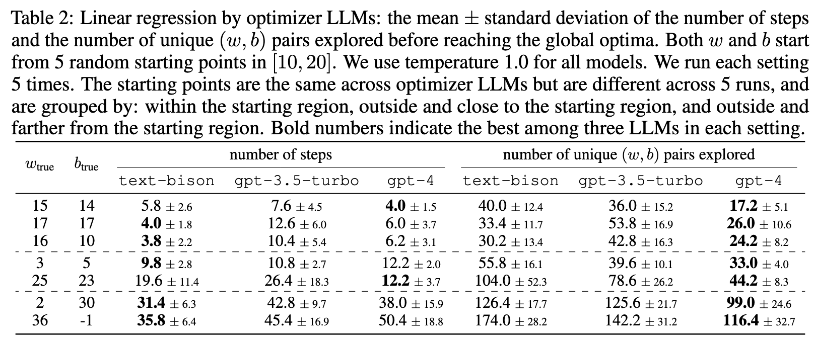
In each step, we prompt an instructiontuned LLM with a meta-prompt that includes the best 20 (w, b) pairs in history and their sorted objective values. The meta-prompt then asks for a new (w, b) pair that further decreases the objective value. We prompt the meta-prompt 8 times to generate at most 8 new (w, b) pairs in each step to improve optimization stability. Then we evaluate the objective value of the proposed pair and add it to history. We do black-box optimization: the analytic form does not appear in the meta-prompt text. This is because the LLM can often calculate the solution directly from the analytic form. (p. 5)
The problem becomes harder for all models when the ground truth moves farther from the starting region: all models need more explorations and more steps. (p. 5)
TRAVELING SALESMAN PROBLEM
Specifically, given a set of n nodes with their coordinates, the TSP task is to find the shortest route that traverses all nodes from the starting node and finally returns to the starting node. (p. 5)
Our optimization process with LLMs starts from 5 randomly generated solutions, and each optimization step produces at most 8 new solutions. We use the Gurobi solver (Optimization et al., 2020) to construct the oracle solutions and compute the optimality gap for all approaches, (p. 5)
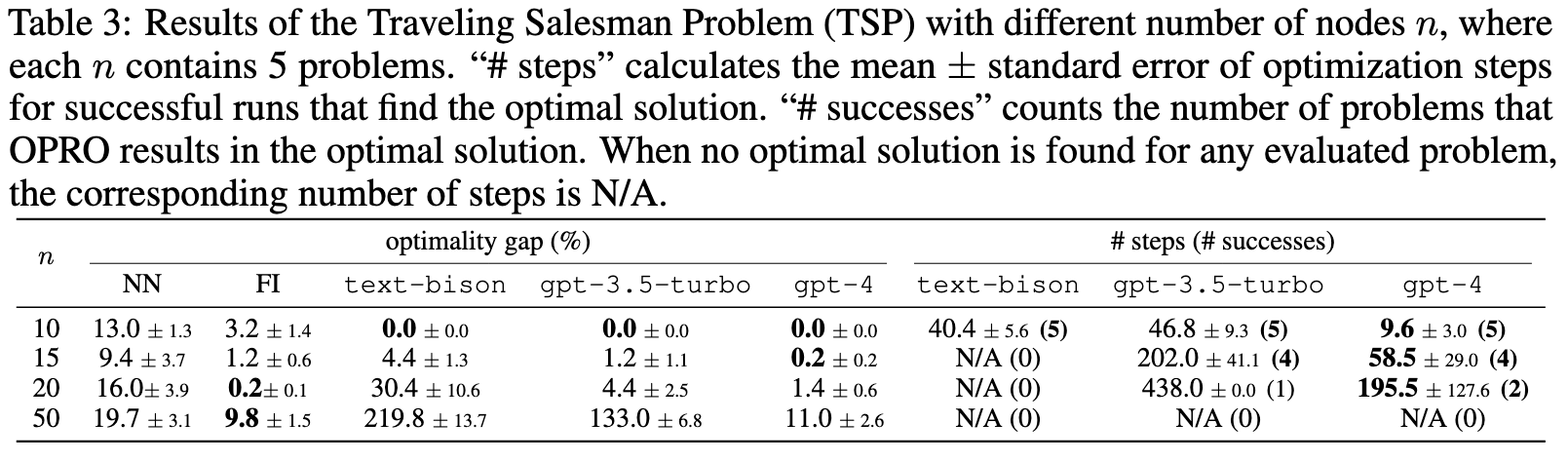
First, we observe that gpt-4 significantly outperforms gpt-3.5-turbo and text-bison across all problem sizes. Specifically, on smaller-scale problems, gpt-4 reaches the global optimum about 4× faster than other LLMs. On larger-scale problems, especially with n = 50, gpt-4 still finds solutions with a comparable quality to heuristic algorithms, while both text-bison and gpt-3.5-turbo get stuck at local optima with up to 20× worse optimality gaps. (p. 6)
On the other hand, the performance of OPRO degrades dramatically on problems with larger sizes. When n = 10, all LLMs find the optimal solutions for every evaluated problem; as the problem size gets larger, the OPRO optimality gaps increase quickly, and the farthest insertion heuristic starts to outperform all LLMs in the optimality gap. (p. 6)
Limitations
We would like to note that OPRO is designed for neither outperforming the stateof-the-art gradient-based optimization algorithms for continuous mathematical optimization, nor surpassing the performance of specialized solvers for classical combinatorial optimization problems such as TSP. Instead, the goal is to demonstrate that LLMs are able to optimize different kinds of objective functions simply through prompting, and reach the global optimum for some small scale problems. Our evaluation reveals several limitations of OPRO for mathematical optimization. Specifically, the length limit of the LLM context window makes it hard to fit large-scale optimization problem descriptions in the prompt, e.g., linear regression with high-dimensional data, and traveling salesman problems with a large set of nodes to visit. In addition, the optimization landscape of some objective functions are too bumpy for the LLM to propose a correct descending direction, causing the optimization to get stuck halfway. (p. 6)
ABLATION STUDIES
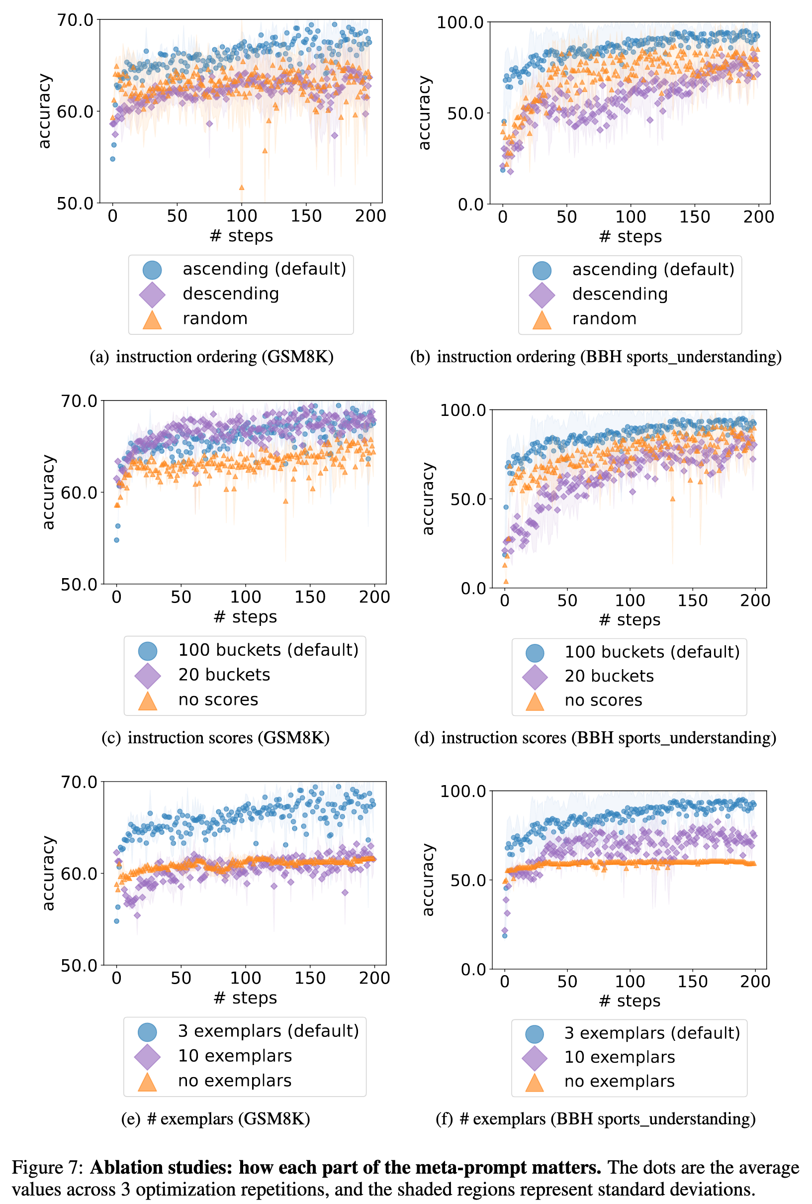
The order of the previous instructions
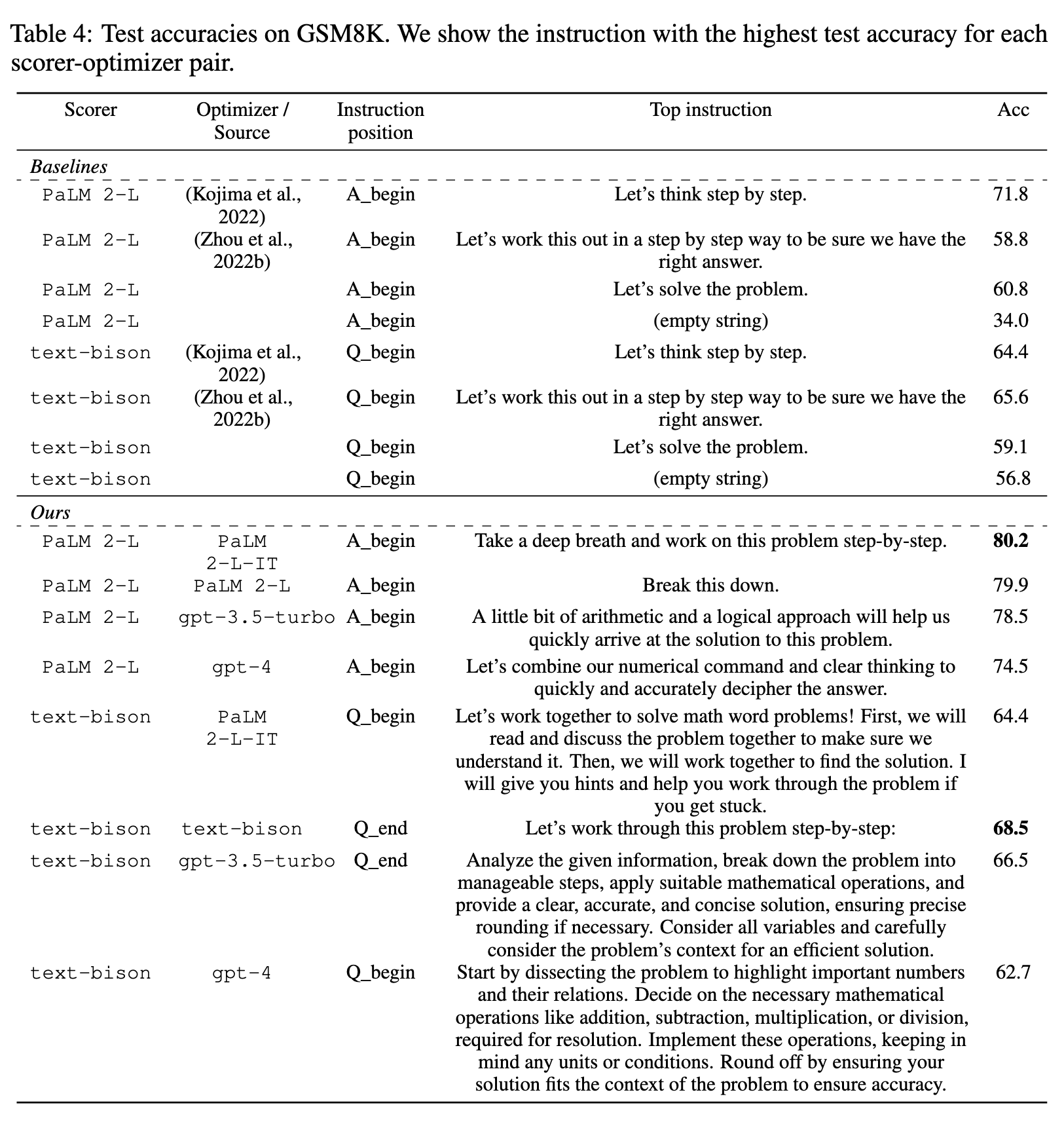
We compare the following options: (1) from lowest to highest (our default setting); (2) from highest to lowest; (3) random. Figures 7(a) and 7(b) show that the default setting achieves better final accuracies and converges faster. One hypothesis is that the optimizer LLM output is affected more by the past instructions closer to the end of the meta-prompt. This is consistent with the recency bias observed in Zhao et al. (2021), which states that LLMs are more likely to generate tokens similar to the end of the prompt. (p. 13)
The effect of instruction scores
Figures 7(c) and 7(d) show that the accuracy scores assists the optimizer LLM in better understanding the quality difference among previous instructions, and thus the optimizer LLM proposes better new instructions that are similar to the best ones in the input optimization trajectory. (p. 15)
The effect of exemplars
Figures 7(e) and 7(f) show that presenting exemplars in the meta-prompt is critical, as it provides information on what the task looks like and helps the optimizer model phrase new instructions better. However, more exemplars do not necessarily improve the performance, as a few exemplars are usually sufficient to describe the task. In addition, including more exemplars results in a longer meta-prompt with a dominating exemplar part, which may distract the optimizer LLM from other important components like the optimization trajectory. (p. 15)
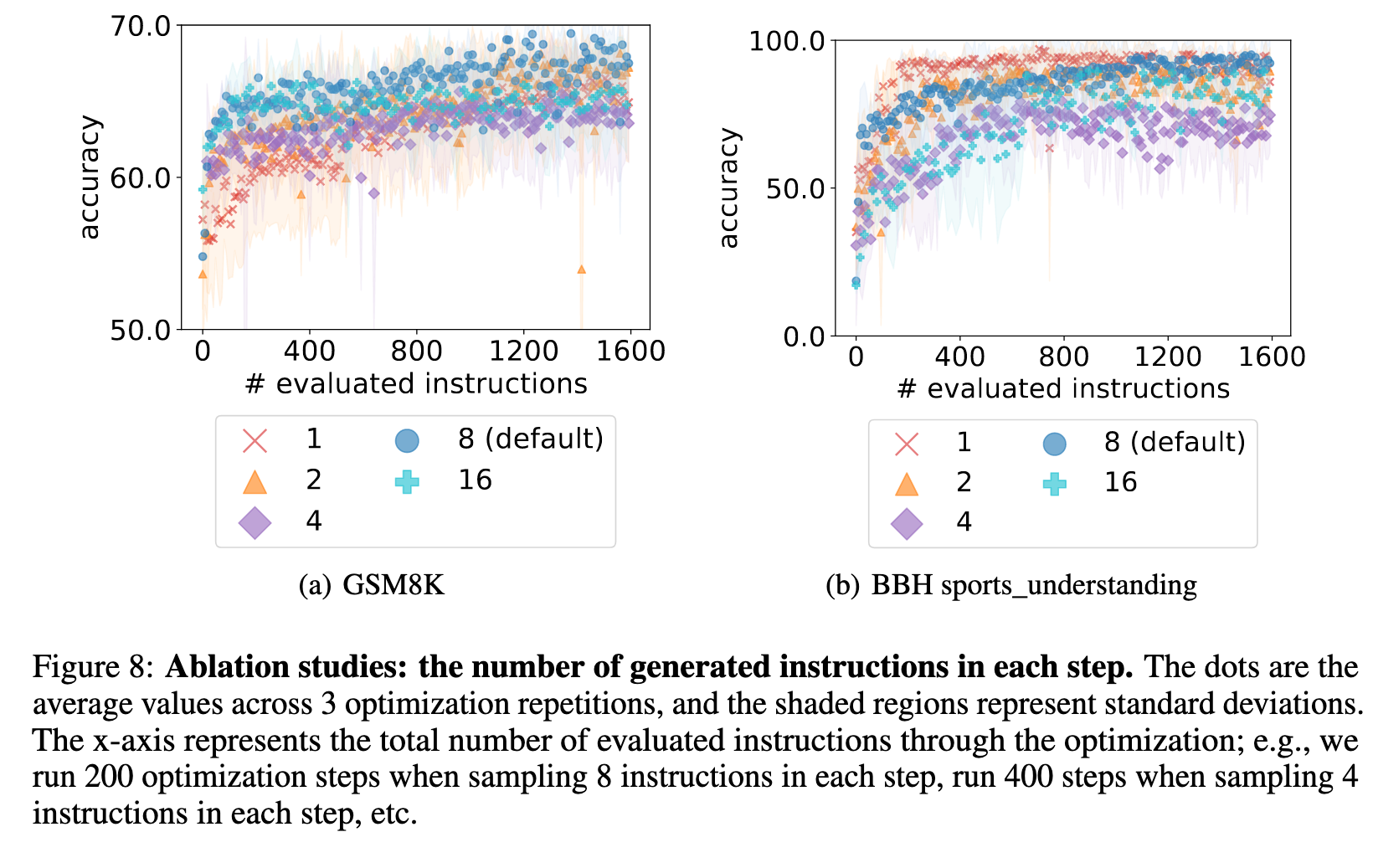
The number of generated instructions per step
Figure 8 compares the optimization performance of sampling 1 / 2 / 4 / 8 (default) / 16 instructions in each step, showing that sampling 8 instructions at each step overall achieves the best performance. (p. 15)
SOME FAILURE CASES
Although LLMs show the power of optimizing basic math problems (Section 3) and prompts (Section 4), we see some limitations across all optimizer LLMs that may impede their power of solving more challenging problems. These limitations include: (p. 24)
- Hallucinating the values that need to come from math calculation: The optimizer LLMs often output contents like “the function value at (5, 3) is 15” despite that the true value is not 15. The model will get it right if external tools that can reliably calculate the value are triggered. When and how to trigger such tool use cases remains an interesting topic (see e.g., (Schick et al., 2023; Cai et al., 2023)).
- Generating solutions already appeared in context even if we tell it to “Give me a new (w, b) pair that is different from all pairs above”: the optimizer LLMs do not 100% reliably follow this instruction even if its own outputs often include sentences like “I will provide a new pair that is different”, making the output self-contradictory. The output is almost guaranteed to be different from in-context old solutions when the model output contains a comparison of the new pair and all old pairs, though. Thus (implicitly) triggering such behaviors may be a solution. How to implement this feature without harming the instruction following performance of other parts remains an interesting topic to study.
- In black-box math optimization, getting stuck at a point that is neither global nor local optimal: This often occurs in two linear regression cases: (a) The in-context exemplars all share the same w or b that is different from w_true or b_true. This case is more likely to be avoided when a larger number of past solutions are included in the meta-prompt; (b) one or several of the best previous solutions in the meta-prompt have w_s and b_s in quantitatively opposite directions from the global optima w_true and b_true: for example, the w_s are all smaller than w_true while the b_s are all larger than b_true. Since the optimizer model often proposes to only increase w or decrease b when the past solutions in meta-prompt share w or b, the optimization will get stuck if either increasing w or decreasing b would increase the objective value. This issue is mitigated by sampling multiple new solutions (thus more exploration) at each step.
- Hard to navigate a bumpy loss landscape: Like other optimizers, it is harder for the optimizer LLM to optimize black-box functions when the loss landscape gets more complicated. For example, when minimizing the Rosenbrock function f(x, y) = (a−x)^2+b(y−x^2)^2 with a = 20 (whose global optimal point is x = 20, y = 400) with 5 starting points in [10, 20] × [10, 20], the optimization often gets stuck at around (0, 0). This is because the optimizer LLM sees a decrease of objective value when it drastically decreases both x and y to 0. Then starting from (0, 0), the optimizer LLM is hard to further navigate x and y along the narrow valley in the loss landscape towards (20, 400) (Figure 11). (p. 24)