NeuralField-LDM Scene Generation with Hierarchical Latent Diffusion Models
[ibrnet autoencoder diffusion nerf latent nerfusion deep-learning gaudi hierarchical pixelnerf 3d This is my reading note on NeuralField-LDM Scene Generation with Hierarchical Latent Diffusion Models. It trains auto-encoder to project RGB images of scene with camera pose into the latent space (voxel-nerf). It uses three levels of latent to represent the scene and then uses hierarchical latent diffusion model to represent it.
Introduction
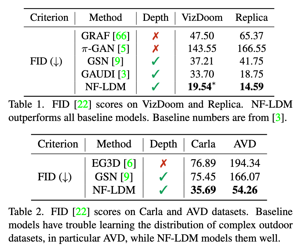
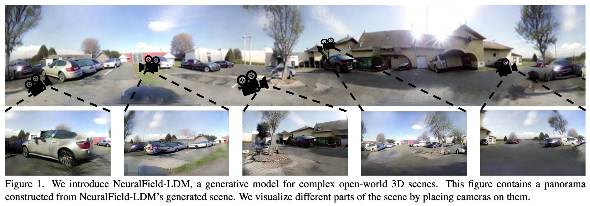
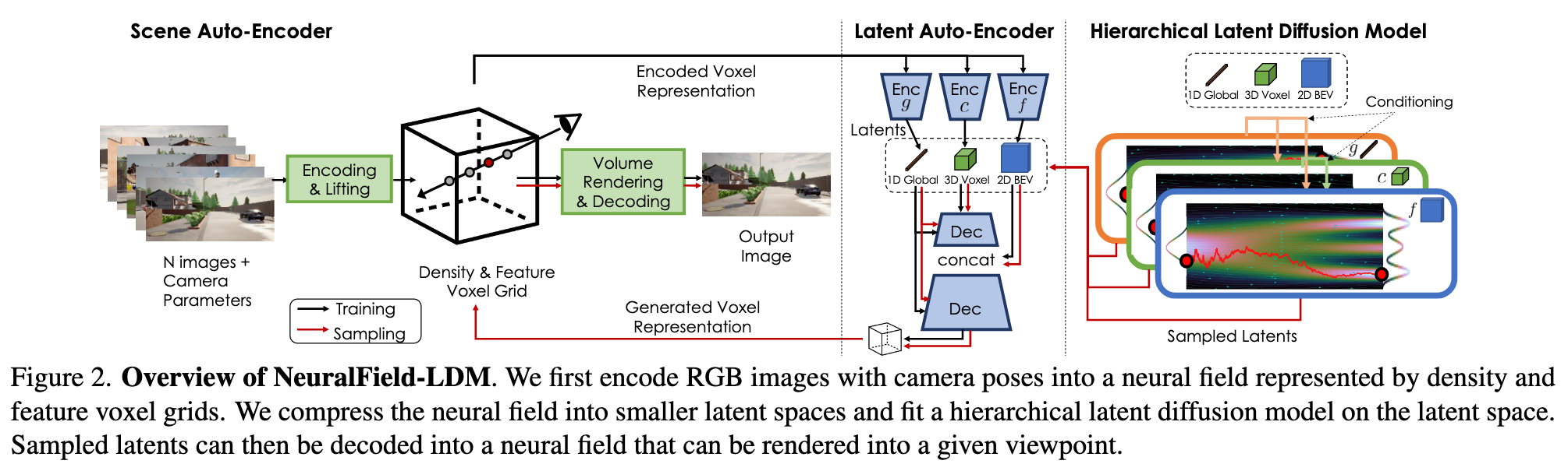
Towards this goal, we introduce NeuralField-LDM, a generative model capable of synthesizing complex 3D environments. We leverage Latent Diffusion Models that have been successfully utilized for efficient high-quality 2D content creation. We first train a scene auto-encoder to express a set of image and pose pairs as a neural field, represented as density and feature voxel grids that can be projected to produce novel views of the scene. To further compress this representation, we train a latent-autoencoder that maps the voxel grids to a set of latent representations. A hierarchical diffusion model is then fit to the latents to complete the scene generation pipeline. We achieve a substantial improvement over existing state of-the-art scene generation models (p. 1)
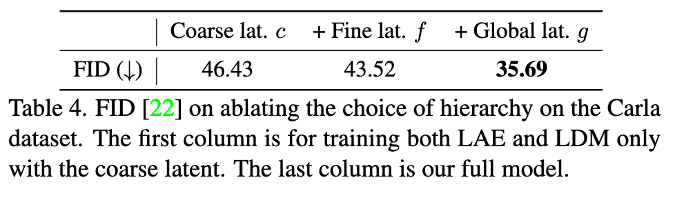
Specifically, a latent-autoencoder decomposes the scene voxels into a 3D coarse, 2D fine and 1D global latent. Hierarchichal diffusion models are then trained on the tri-latent representation to generate novel 3D scenes (p. 2)
PixelNeRF [84] and IBRNet [82] propose to condition NeRF on aggregated features from multiple views to enable novel view synthesis from a sparse set of views. Another line of works scale NeRF to large-scale indoor and outdoor scenes [46, 57, 86, 88]. Recently, Nerfusion [88] predicts local radiance fields and fuses them into a scene representation using a recurrent neural network (p. 2)
The work closest to ours is GAUDI [3], which first trains an auto-decoder and subsequently trains a DDM on the learned latent codes. Instead of using a global latent code, we encode scenes onto voxel grids and train a hierarchical DDM to optimally combine global and local features. (p. 2)
Proposed Method
Scene Auto-Encoder
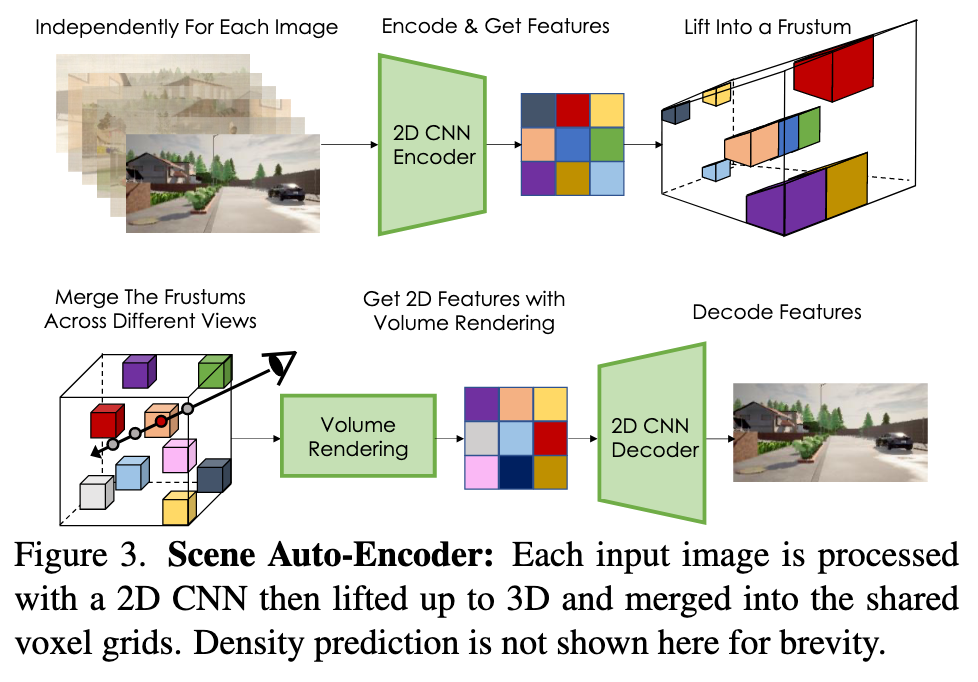
We follow a similar procedure to LiftSplat-Shoot (LSS) [52] to lift each 2D image feature map and combine them in the common voxel-based 3D neural field. We build a discrete frustum of size H × W × D with the camera poses κ for each image. This frustum contains image features and density values for each pixel, along a pre-defined discrete set of D depths. (p. 3)
That is, the d’th channel of the CNN’s output at pixel (h, w) becomes the density value of the frustum entry at (h, w, d). (p. 3)

For each voxel indexed by (x, y, z), we pool all densities and features of the corresponding frustum entries. In this paper, we simply take the mean of the pooled features. More sophisticated pooling functions (e.g. attention) can be used, which we leave as future work. (p. 3)
Finally, we perform volume rendering using the camera poses κ to project V onto a 2D feature map. We trilinearly interpolate the values on each voxel to get the feature and density for each sampling point along the camera rays. 2D features are then fed into a CNN decoder that produces the output image ˆi. (p. 3)
| auto-encoding pipeline is trained with an image reconstruction loss | i − ˆi | and a depth supervision loss | ρ − ρˆ | . (p. 4) |
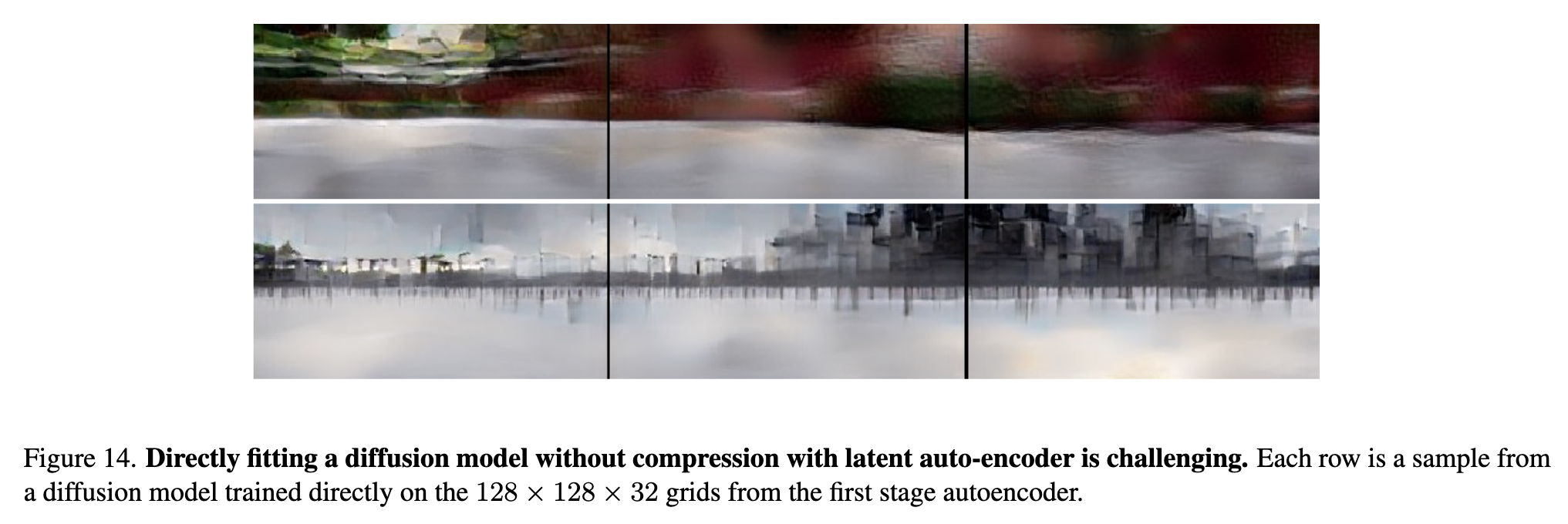
We hypothesize that current DMs cannot perform well on very high dimensional data, highlighting the importance of our hierarchical latent space. Tab. 12 reports perceptual loss on reconstructed output viewpoints. We concluded that 128 × 128 × 32 provides a satisfactory output quality while still being small enough for the consequent stages to model and to not consume excessive GPU memory. (p. 19)
Latent Voxel Auto-Encoder
We thus introduce a latent auto-encoder (LAE) that compresses voxels into a 128dimensional global latent as well as coarse (3D) and fine (2D) quantized latents with channel dimensions of four and spatial dimensions 32×32×16 and 128×128 respectively. (p. 4)
We concatenate V_Density and V_Feat along the channel dimension and use separate CNN encoders to encode the voxel grid V into a hierarchy of three latents: 1D global latent g, 3D coarse latent c, and 2D fine latent f, as shown in Fig. 12. The intuition for this design is that g is responsible for representing the global properties of the scene, such as the time of the day, c represents coarse 3D scene structure, and f is a 2D tensor with the same horizontal size X × Y as V , which gives further details for each location (x, y) in bird’s eye view perspective. We empirically found that 2D CNNs perform similarly to 3D CNNs while being more efficient, thus we use 2D CNNs throughout. To use 2D CNNs for the 3D input V , we concatenate V ’s vertical axis along the channel dimension and feed it to the encoders. We also add latent regularizations to avoid high variance latent spaces [60]. For the 1D vector g, we use a small KL-penalty via the reparameterization trick [38], and for c and f, we impose a vector-quantization [15,80] layer to regularize them. (p. 4)
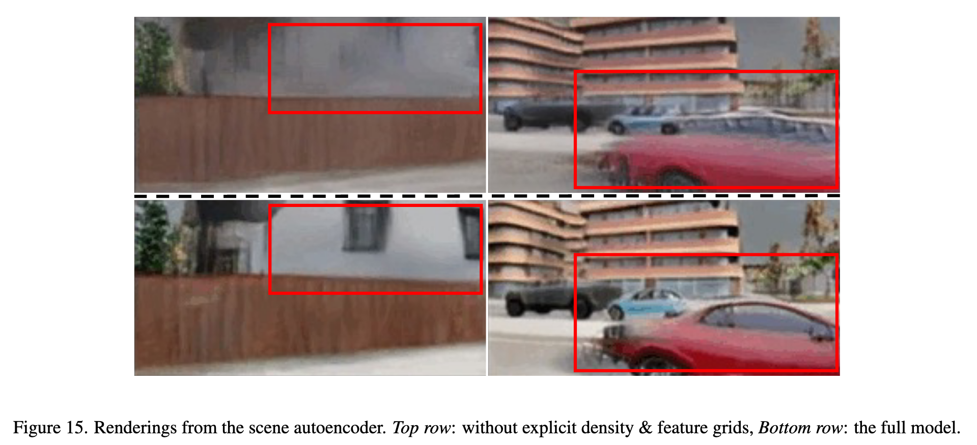
Explicit Density: in Fig. 15, we show that having explicit feature and density grids outperforms implicitly inferring density from the voxel features with an MLP. (p. 19)
Hierarchical Latent Diffusion Models
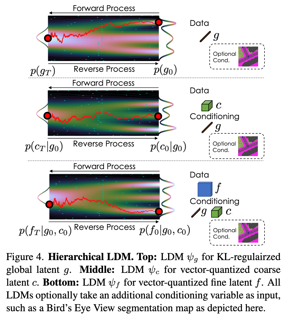
| Given the latent variables g, c, f that represent a voxelbased scene representation V , we define our generative model as p(V, g, c, f) = p(V | g, c, f)p(f | g, c)p(c | g)p(g) with Denoising Diffusion Models (DDMs) [24]. (p. 4) |
The camera poses contain the trajectory the camera is travelling, and this information can be useful for modelling a 3D scene as it tells the model where to focus on generating. Therefore, we concatenate the camera trajectory information to g and also learn to sample it. For brevity, we still call the concatenated vector g. For conditional generation, each ψ takes the conditioning variable as input with cross-attention layers [60]. (p. 5)
We found that ds = 4 gives a good compromise between having a low reconstruction loss and a latent size small enough to fit a diffusion model. (p. 19)
Post-Optimizing Generated Neural Fields
Specifically, we iteratively update initially generated voxels, V , by rendering viewpoints from the scene and applying Score Distillation Sampling (SDS) [53] loss on each image independently (p. 5)
For ϵˆθ, we use an off-the-shelf latent diffusion model [60], finetuned to condition on CLIP image embeddings [54]1. We found that CLIP contains a representation of the quality of images that the LDM is able to interpret: denoising an image while conditioning on CLIP image embeddings of our model’s samples produced images with similar geometry distortions and texture errors. We leverage this property by optimizing LSDS with negative guidance. Letting y, y′ be CLIP embeddings of clean image conditioning (e.g. dataset images) and artifact conditioning (e.g. samples) respectively, we perform classifier-free guidance [26] with conditioning vector y, but replace the unconditional embedding with y′. (p. 5)
Experiments