unCLIP-Hierarchical Text-Conditional Image Generation with CLIP Latents
[multimodality clip dalle2 diffusion text-image glide dall-e2 deep-learning image-synthesize unclip dall-e This is my reading note on Hierarchical Text-Conditional Image Generation with CLIP Latents. This paper proposes a two-stage model (unCLIP): a prior that generates a CLIP image embedding given a text caption, and a decoder that generates an image conditioned on the image embedding, for generating images from text.
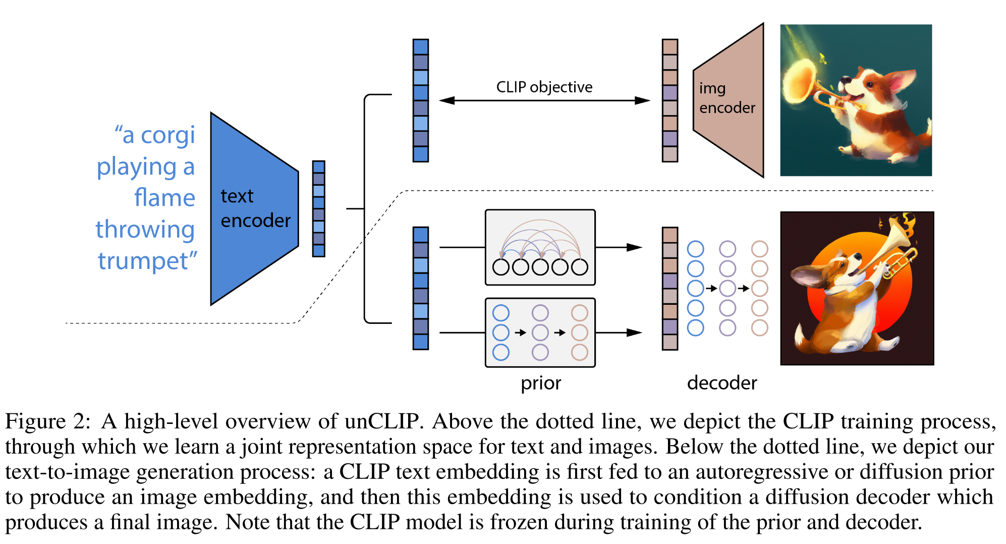
The overview of unCLIP is shown below. The part above is training process which is based on CLIP to train the image encoder and text encoder that aligns to the same space. It requires pairs of text (y) and image (x). The text encoder and image encoder generates the text embedding \(z_t\) and image embedding \(z_i\) accordingly.
| The part below is the inference process, where the prior could be autoregressor or diffusion, and decoder is diffusion model. The process of generating image x from text y could be written as $$p(x | y)=p(x,z_i | y)=p(x | z_i,y)p(z_i | y)$$ |
CLIP
CLIP embeddings have a number of desirable properties:
- they are robust to image distribution shift,
- have impressive zero-shot capabilities,
- and have been fine-tuned to achieve state-of-the-art results on a wide variety of vision and language tasks [45].
Decoder
We use diffusion models [25, 48] to produce images conditioned on CLIP image embeddings (and optionally text captions). Specifically, we modify the architecture described in GLIDE by projecting and adding CLIP embeddings to the existing timestep embedding, and by projecting CLIP embeddings into four extra tokens of context that are concatenated to the sequence of outputs from the GLIDE text encoder. We retained the text conditioning pathway present in the original GLIDE model, hypothesizing that it could allow the diffusion model to learn aspects of natural language that CLIP fails to capture (e.g. variable binding), but find that it offers little help in this regard (Section 7).
We enable classifier-free guidance [24] by randomly setting the CLIP embeddings to zero (or a learned embedding) 10% of the time, and randomly dropping the text caption 50% of the time during training. To generate high resolution images, we train two diffusion upsampler models [34, 43]: one to upsample images from 64×64 to 256×256 resolution, and another to further upsample those to 1024×1024 resolution. To improve the robustness of our upsamplers, we slightly corrupt the conditioning images during training. For the first upsampling stage, we use gaussian blur [43], and for the second, we use a more diverse BSR degradation [42, 59].
Prior
While a decoder can invert CLIP image embeddings \(z_i\) to produce images x, we need a prior model that produces \(z_i\) from captions y to enable image generations from text captions. We explore two different model classes for the prior model:
- Autoregressive (AR) prior: the CLIP image embedding \(z_i\) is converted into a sequence of discrete codes and predicted autoregressively conditioned on the caption y. We condition the AR prior on the text caption and the CLIP text embedding by encoding them as a prefix to the sequence. Additionally, we prepend a token indicating the (quantized) dot product between the text embedding and image embedding, \(z_i\cdot z_t\).
- Diffusion prior: The continuous vector \(z_i\) is directly modelled using a Gaussian diffusion model conditioned on the caption y. For the diffusion prior, we train a decoder-only Transformer with a causal attention mask on a sequence consisting of, in order: the encoded text, the CLIP text embedding, an embedding for the diffusion timestep, the noised CLIP image embedding, and a final embedding whose output from the Transformer is used to predict the unnoised CLIP image embedding.
To train and sample from the AR prior more efficiently, we first reduce the dimensionality of the CLIP image embeddings zi by applying Principal Component Analysis (PCA) [37]. We are able to preserve nearly all of the information2 by retaining only 319 principal components out of the original 1,024.
Image Manipulations
Our approach allows us to encode any given image x into a bipartite latent representation \((z_i, x_T)\) that is sufficient for the decoder to produce an accurate reconstruction. The latent \(z_i\) describes the aspects of the image that are recognized by CLIP, while the latent \(x_T\) encodes all of the residual information necessary for the decoder to reconstruct x. The former is obtained by simply encoding the image with the CLIP image encoder. The latter is obtained by applying DDIM inversion (Appendix F in [11]) to x using the decoder, while conditioning on \(z_i\). We describe three different kinds of manipulations that are enabled by this bipartite representation.
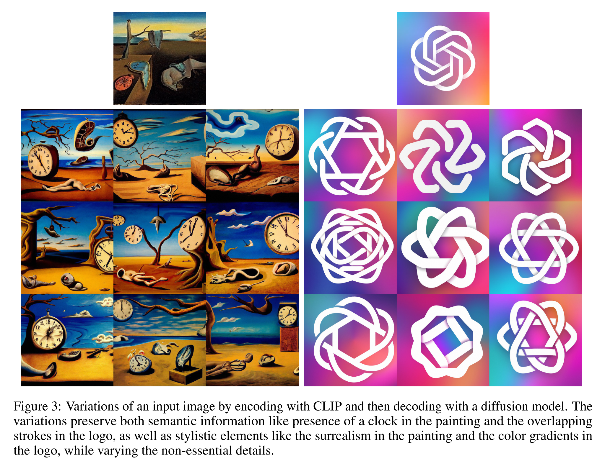
Variations
Given an image x, we can produce related images that share the same essential content but vary in other apects, such as shape and orientation (Figure 3). To do this, we apply the decoder to the bipartite representation \((z_i, x_T)\) using DDIM with \(\eta\gt0\) for sampling. With \(\eta=0\), the decoder becomes deterministic and will reconstruct the given image x. Larger values of η introduce stochasticity into successive sampling steps, resulting in variations that are perceptually “centered” around the original image x. As
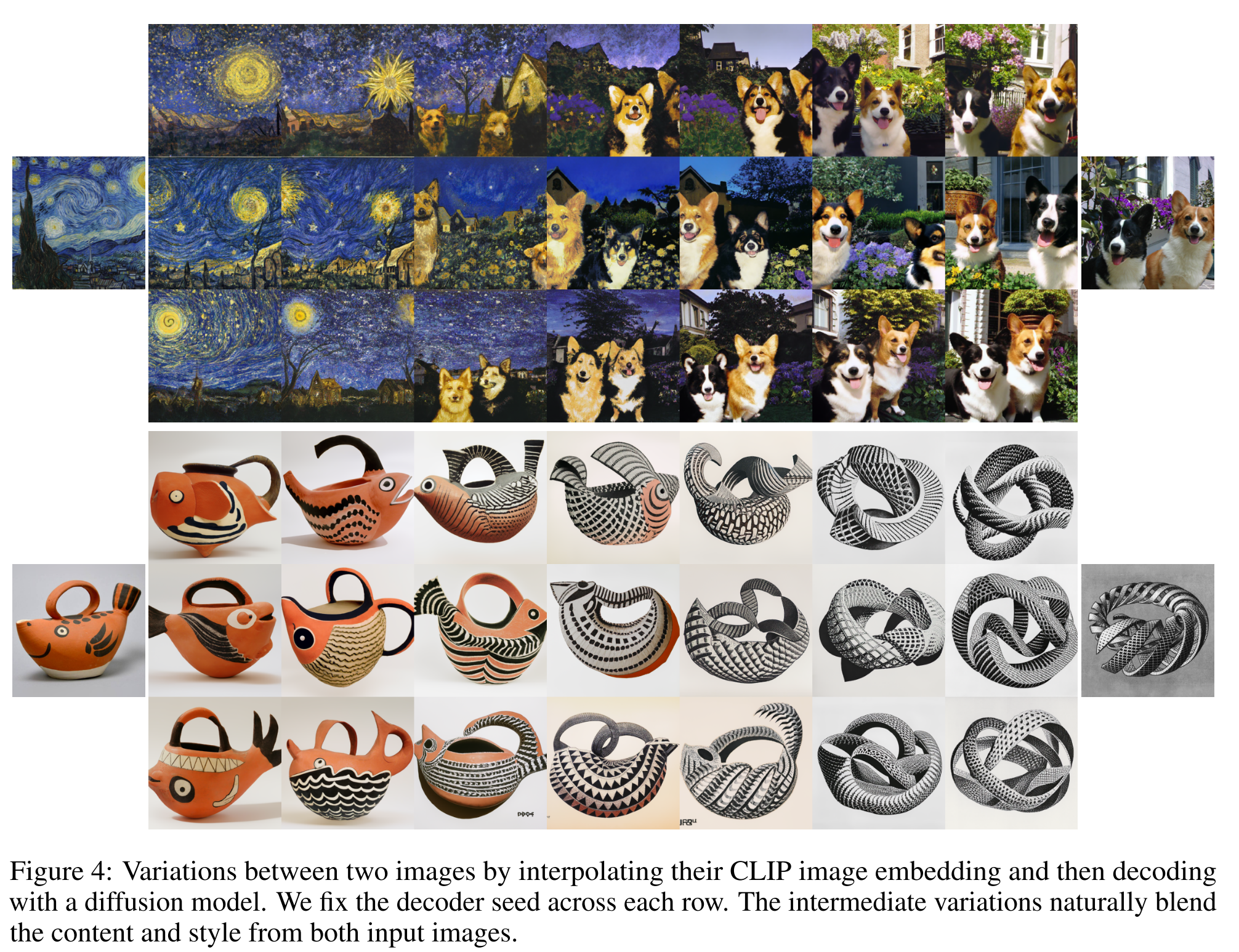
Interpolations
It is also possible to blend two images \(x_1\) and \(x_2\) for variations (Figure 4), traversing all of the concepts in CLIP’s embedding space that occur between them. To do this, we rotate between their CLIP embeddings \(z_{i_1}\) and \(z_{i_2}\) using spherical interpolation, yielding intermediate CLIP representations \(z_{i_\theta} = slerp(z_{i_1}, z_{i_2} , \theta)\) as \(\theta\) is varied from 0 to 1.
There are two options for producing the intermediate DDIM latents along the trajectory. The first option involves interpolating between their DDIM inverted latents \(x_{T_1}\) and \(x_{T_2}\) (by setting \(x_{T_\theta} = slerp(x_{T_1}, x_{T_2} , \theta))\), which yields a single trajectory whose endpoints reconstruct \(x_1\) and \(x_2\). The second option involves fixing the DDIM latent to a randomly-sampled value for all interpolates in the trajectory. This results in an infinite number of trajectories between \(x_1\) and \(x_2\), though the endpoints of these trajectories will generally no longer coincide with the original images.
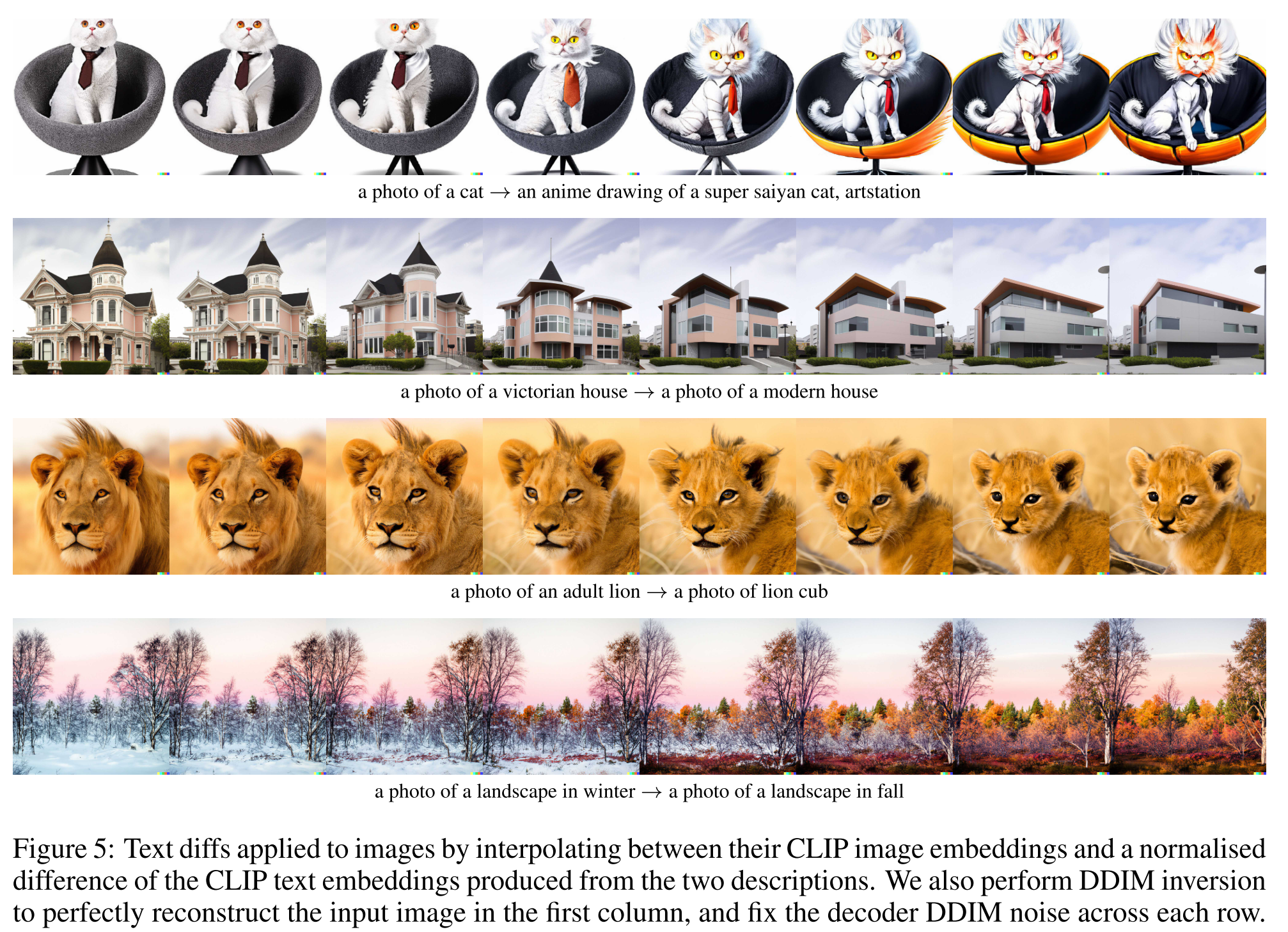
Text Diffs
To modify the image to reflect a new text description y, we first obtain its CLIP text embedding \(z_t\), as well as the CLIP text embedding \(z_{t_0}\) of a caption describing the current image4. We then compute a text diff vector \(z_d = norm(z_t − z_{t_0} )\) from these by taking their difference and normalizing. Now, we can rotate between the image CLIP embedding \(z_i\) and the text diff vector \(z_d\) using spherical interpolation, yielding intermediate CLIP representations \(z_\theta = slerp(z_i, z_d, \theta)\), where \(\theta\) is increased linearly from 0 to a maximum value that is typically in [0.25, 0.50].